Constructing a bootstrap confidence interval in Julia

1 March 2025

I was reading a blog post that gave an example of where the frequentist approach differs from the Bayesian approach.

The post presents the example of drawing a sample of nine data points from a Bernoulli distribution and we want to estimate the parameter \(p\) which represent the probability of seeing a success. Say we see one success and eight failures, our maximum likelihood estimate for \(p\) is just the proportion of success cases we see in our sample and here that is \(\hat{p} = \frac{1}{1 + 8} = \frac{1}{9}\).

Naturally, we may want to add a confidence interval to quantify our uncertainty about our estimate since depending on what values we happened sampled we could have come up with a value for \(\hat p\) that’s slightly bigger or smaller.

A natural first step is to estimate the standard error of the distribution as we typically do for similar problems which in this case we know is \(\hat{\sigma} = \hat{p} (1 - \hat{p})\).

The sampling distribution is the hypothetical distribution that we would see if we applied our estimator to randomly generated samples of the same size as our observation from the real distribution of our population. The blog post then presents the sampling distribution of our parameter estimate as \(\mathcal{N}(\hat{p}, \hat{\sigma})\).

I wrote some Julia code to visualise it

using Distributions
using Plots
d = Binomial(9, 0.11)
p̂ = rand(d) / 9
σ̂ = p̂ * (1 - p̂)
p̂_d = Normal(p̂, σ̂)
xs = LinRange(-0.5, 0.5, 10_000)
plot(xs, pdf(p̂_d, xs), lab="Likelihood")

forbidden = LinRange(-0.5, 0, 10_000)
plot!(
  forbidden,
  pdf(p̂_d, forbidden),
  ribbon=(pdf(p̂_d, forbidden), 0),
  lab="Impossible",
  ylab="Density",
  xlab="\$p\$"
)

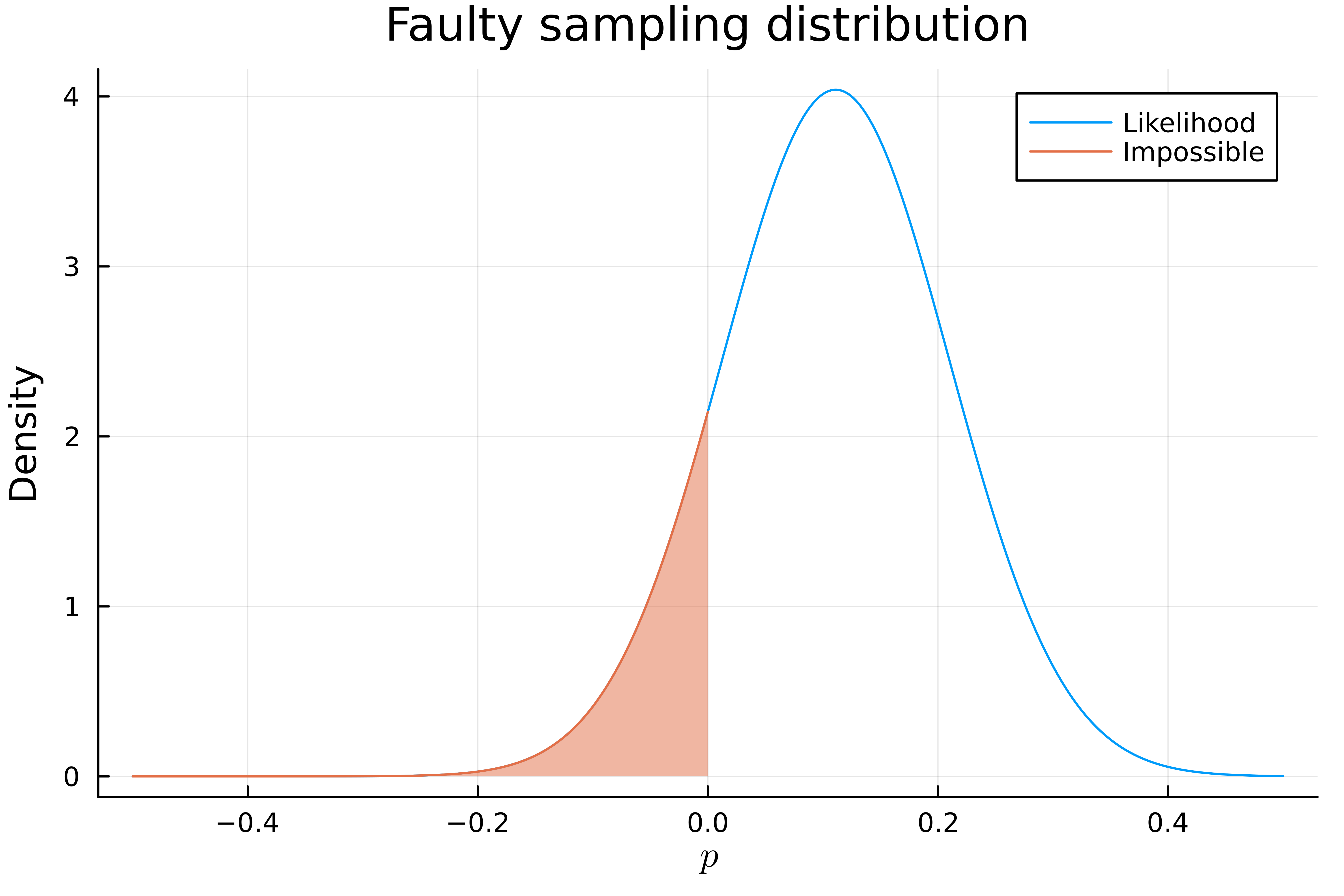
There is a clear problem here since our distribution for \(\hat{p}\) contains values which are negative which is impossible for \(p\) since it represents a probability. In fact, about 20% of our supposed sampling distribution is negative!

The mistake here was approximating the sampling distribution of our estimate with a normal distribution. Since our sample size is so small and \(\hat p\) is so close to 0 this approximation is just inaccurate.

The blog post doesn’t mention it but we can instead construct the bootstrap estimate for the confidence interval.

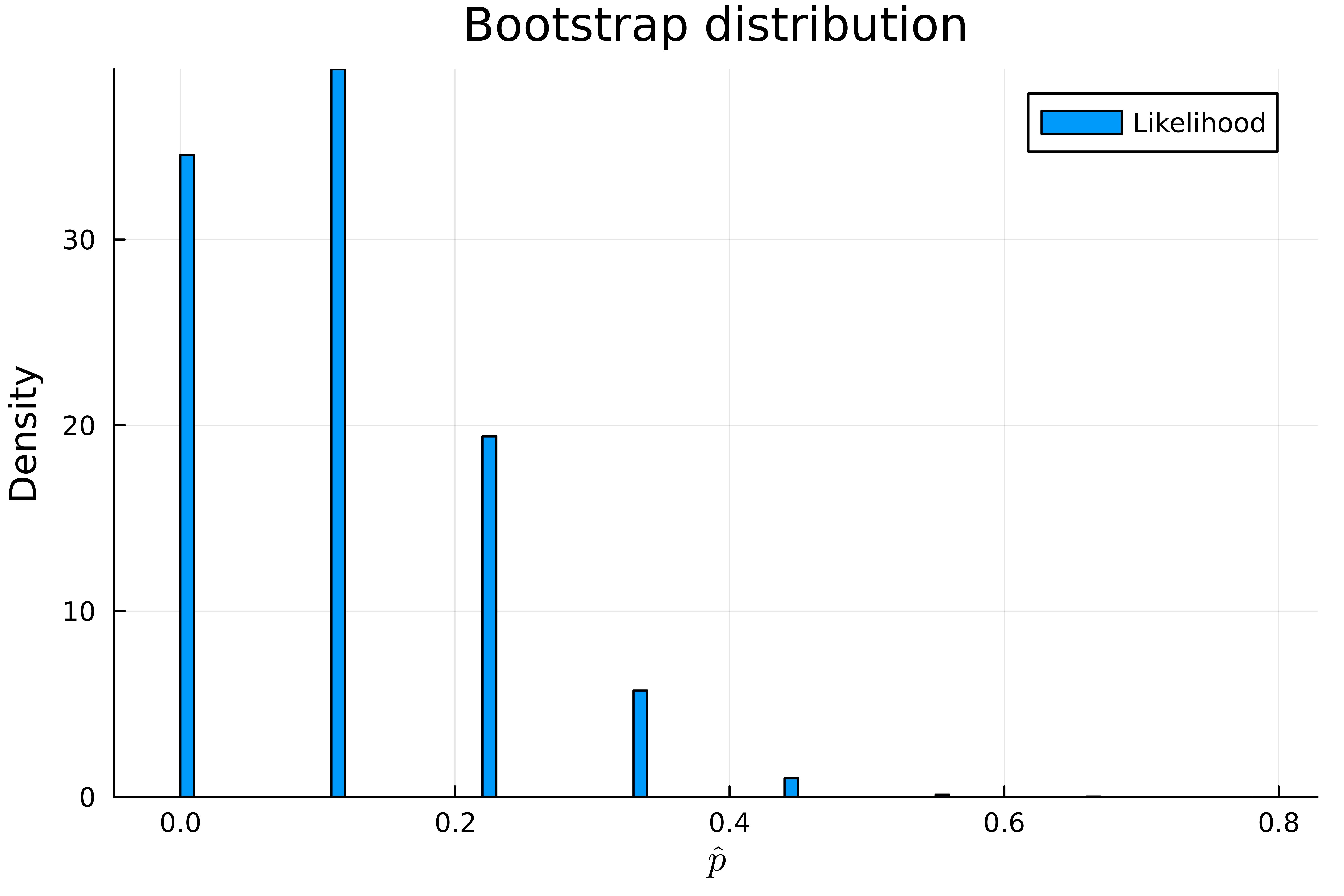
Case resampling bootstrap works by constructing a series of bootstrap samples by resampling with replacement from our original set of observations and approximating the distribution of our estimate using the values of our estimator on our bootstrap samples. Here our results look far more sensible.

In Julia it looks like this

bootstrap_samples = 100_000
data = [1; zeros(8)]  # 1 success, 8 failures
bootstrap_p̂s = zeros(0)
for _ in 1:bootstrap_samples
    bootstrap_p̂ = sum(rand(data, 9)) / 9
    bootstrap_p̂s = append!(bootstrap_p̂s, bootstrap_p̂)
end
histogram(
  bootstrap_p̂s,
  normalize=true,
  dpi=1000,
  ylab="Density",
  xlab="\$\\hat p\$",
  title="Bootstrap distribution",
  lab="Likelihood"
)

We can also estimate the 95% confidence interval

sorted_p̂s = sort(bootstrap_p̂s)
lower = sorted_p̂s[Int(ceil(0.025 * bootstrap_samples))]
upper = sorted_p̂s[Int(ceil(0.975 * bootstrap_samples))]
print("95% Bootstrap CI: [$lower, $upper]")

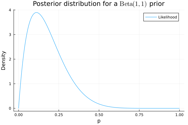
Just for funsies we can also get the Bayesian posterior distribution given a \(\operatorname{Beta}(1, 1)\) prior which represents an indifference between all values of the parameter \(p\). The posterior represents our updated beliefs about \(p\) after exposing ourselves to the data we’ve collected.

bayesian_posterior = Beta(2, 9)
xs = LinRange(0, 1, 10_000)
plot(
  xs,
  pdf(bayesian_posterior, xs),
  xlab="p",
  ylab="Density",
  title="Posterior distribution for a \$\\operatorname{Beta}(1, 1)\$ prior"
)

The blog post has a point though, namely that the Bayesian method is easier to interpret and get right. In my view, the Bayesian posterior has a typically more useful interpretation as our belief for the value of the parameter.

Our bootstrap sampling distribution allocates substantial probability to the case \(\hat{p} = 0\) but we know \(p\) cannot be 0 since in our original sample we observed a success. This happens due to the fact that that, unlike the bayesian posterior, the frequentist confidence interval does not represent our beliefs about the value of the parameter. The confidence interval just represents what our parameter estimate could have been due to randomness in our sampling procedure and when understood this way it’s true that it’s plausible that we could have estimated \(p\) as 0 just by chance.

Our Bayesian posterior assigns \(p = 0\) a probability density of 0 since this case is incompatible with our observation of a success and we could not rationally believe that \(p = 0\) is possible.