Ridge regression: Handling multicollinearity with a Gaussian prior

2 March 2025

I forgot where I first read this but it becomes increasingly hard to estimate coefficients for a linear regression as the predictors become more correlated.

To start with, I’ll sample from multivariate normal distributions with varying covariance. They look like this on a graph

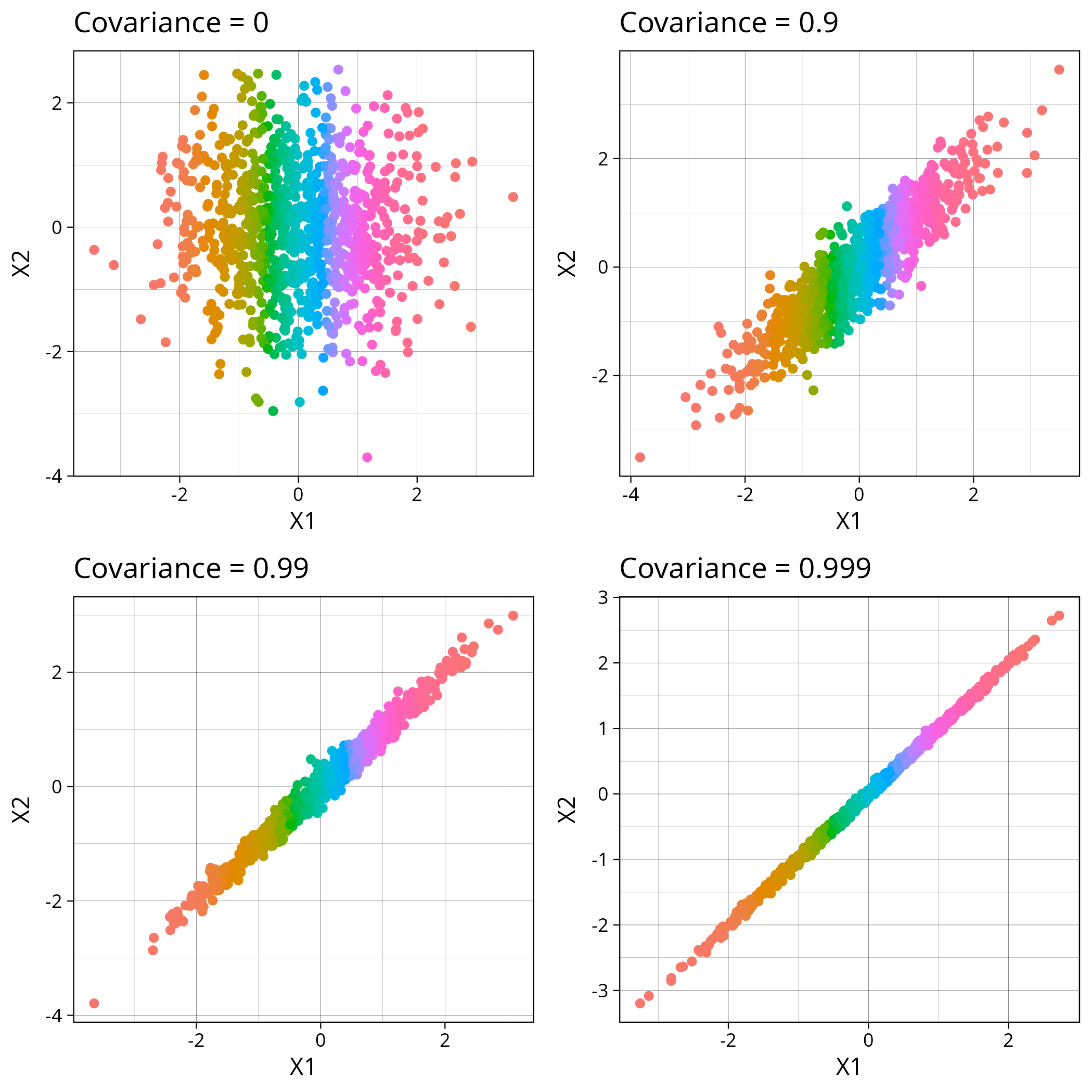
The R code for that looks like this

plot_dist <- function (cov_choice) {
  n <- 1000
  mu <- c(0, 0)
  Sigma <- matrix(c(1, cov_choice, cov_choice, 1), 2, 2)
  df <- data.frame(mvrnorm(n, mu, Sigma))
  ggplot(df) + geom_point(aes(x=X1, y=X2, colour=factor(X1)), show.legend=F) + ggtitle(paste("Covariance =", cov_choice))
}

Next I can fit a linear model. I define the response variable as \(Y = \alpha X_1 + \beta X_2 + \epsilon\) with \(\epsilon \sim \mathcal{N}(0, 1)\). R has a built-in function for fitting linear models called lm and I use it by writing lm(y ~ X1 + X2). My code now looks like this

test_ls <- function (true_alpha, true_beta) {
  covs_to_use <- c(0.99, 0.999, 0.9999, 0.99999, 0.999999)
  covs <- c()
  alphas <- c()
  betas <- c()
  attempts <- c()
  for (cov_value in covs_to_use) {
    for (i in 1:100) {
      n <- 1000
      mu <- c(0, 0)
      Sigma <- matrix(c(1, cov_value, cov_value, 1), 2, 2)
      df <- data.frame(mvrnorm(n, mu, Sigma))
      df$y = true_alpha * df$X1 + true_beta * df$X2 + rnorm(n, 0, 0.1)
      coefficients <- coef(lm(y ~ X1 + X2, df))
      alpha <- coefficients[2]
      beta <- coefficients[3]
      covs <- append(covs, cov_value)
      alphas <- append(alphas, alpha)
      betas <- append(betas, beta)
      attempts <- append(attempts, i)
    }
  }
  data.frame(covariance=covs, alpha=alphas, beta=betas, attempt=attempts)
}

If I set \(\alpha = 0\) and \(\beta = 0\) then \(y\) is just a normally distributed variable that is completely independent of \(X_1\) and \(X_2\). Here are what the least squares estimates for \(\alpha\) look like

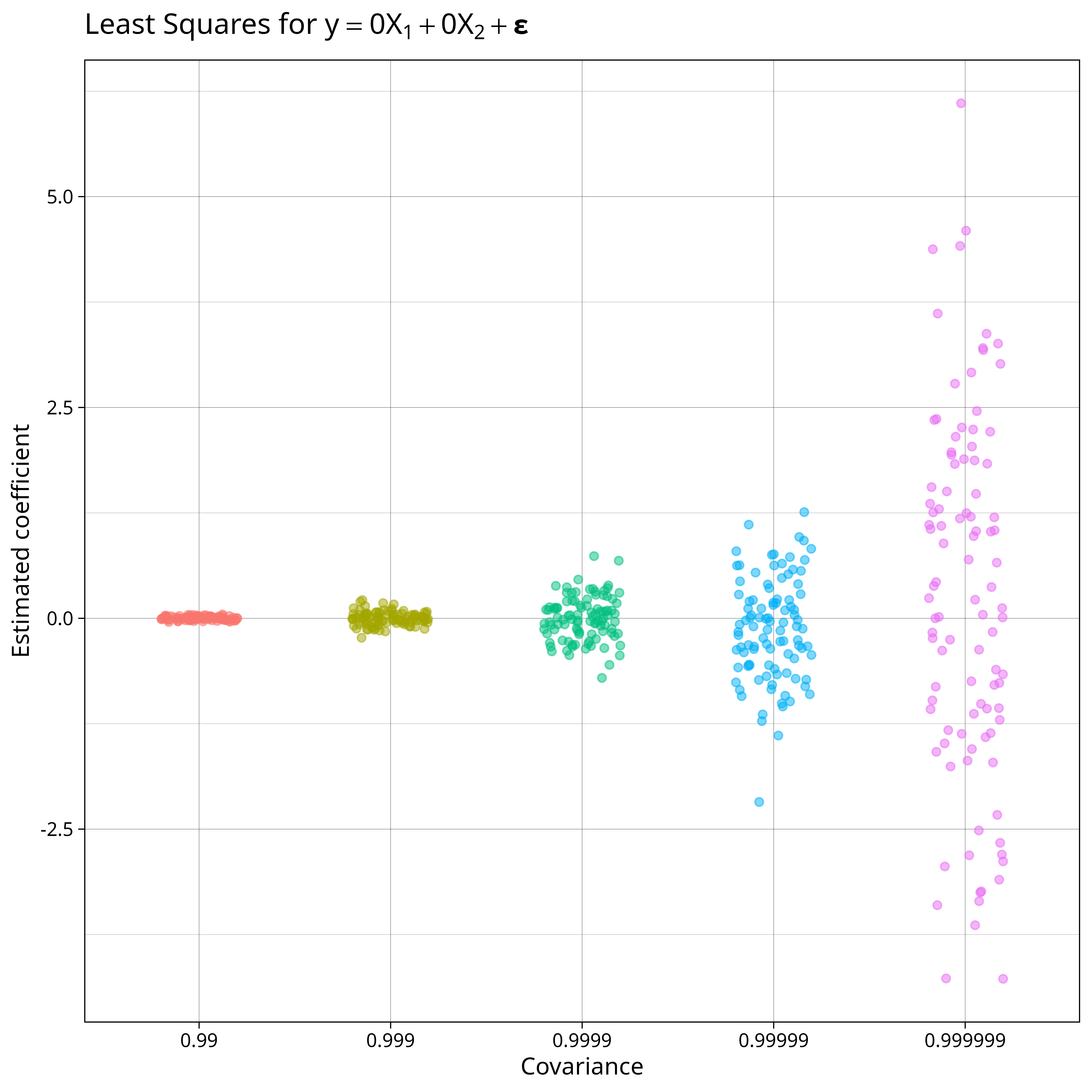
Our estimates for \(\alpha\) worsen as we increase the covariance: there is no relationship between \(y\) and \(X\) but some of our estimates for \(\alpha\) are larger than 4!

Our model is still able to predict well but when our are more correlated it’s difficult to work out how each of our predictors contribute to the final result. If we plot our joint estimates for \(\alpha\) and \(\beta\) on a graph then we consistently get \(\alpha + \beta = 0\) no matter what the covariance is.

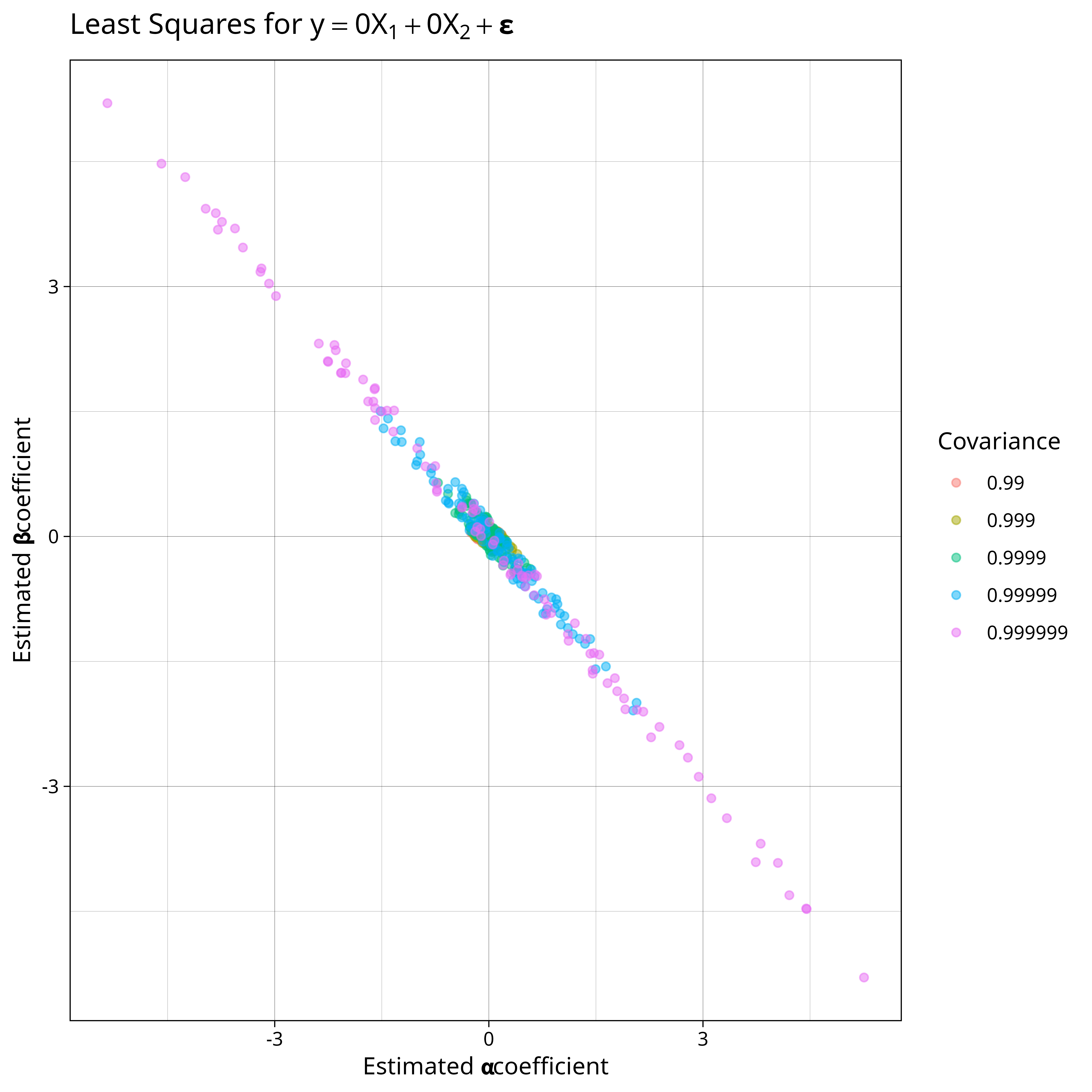
So our model is able to identify \(\alpha + \beta\) but not either of \(\alpha\) and \(\beta\) individually.

We can remedy this by adding a Bayesian prior to our model weights. If we place a prior distribution on our weights then instead of taking the maximum likelihood estimate we can instead find the maximum aposteriori estimate or MAP estimate. The MAP estimate chooses the parameters that maximise our posterior likelihood after observing the data.

If we use a prior of \( w \sim \mathcal{N}( \mathbf{0}, \lambda^{-1} I)\) then after observing data with design matrix \(X\) then we get a MAP estimate of \( (X^\top X + \lambda I)^{-1}X^\top y \). Finding this value is equivalnt to minimising the least-sqaures error with an \(\ell_2\)-penalty which is also known as ridge regression.

The estimation code now looks like this

w <- solve(t(X) %*% X + lambda * diag(2), t(X) %*% df$y)
alpha <- w[1]
beta <- w[2]

And our estimated coefficients look like this

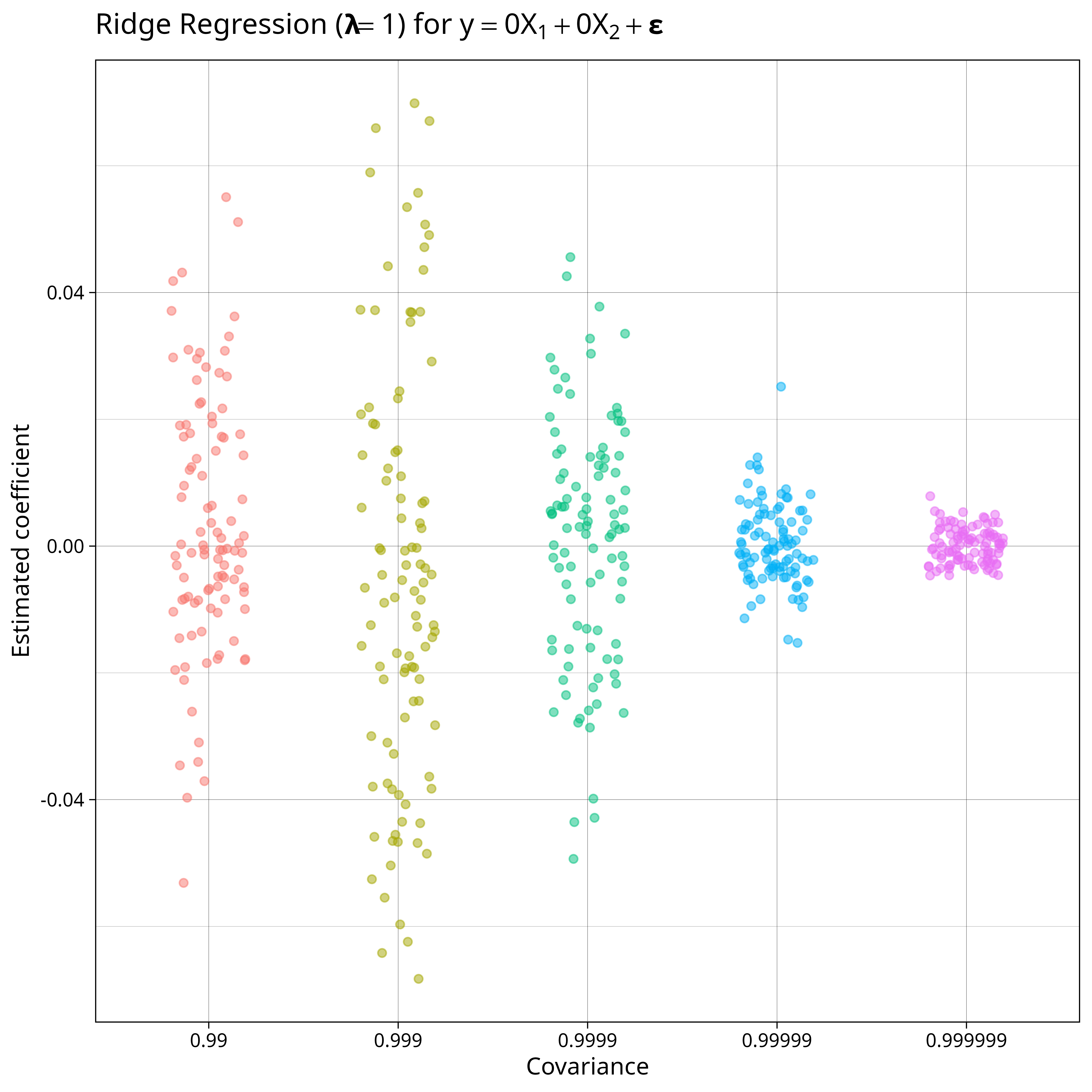
This is much better. We don’t have any wild claims about the predictive effect of our variables and our largest estimate is 0.05. Using a prior gives us the benefit that we use prior knowledge to improve the accuracy of our model. Here we stated that we expected our coefficients to be around 0 and that’s what we see in our MAP.

We can also see what happens when our prior is centred around 0 but the true value of our parameters are non-zero. Here are the plots of the regression results when \(\alpha = 0.2\) and \(\beta = 0.8\)

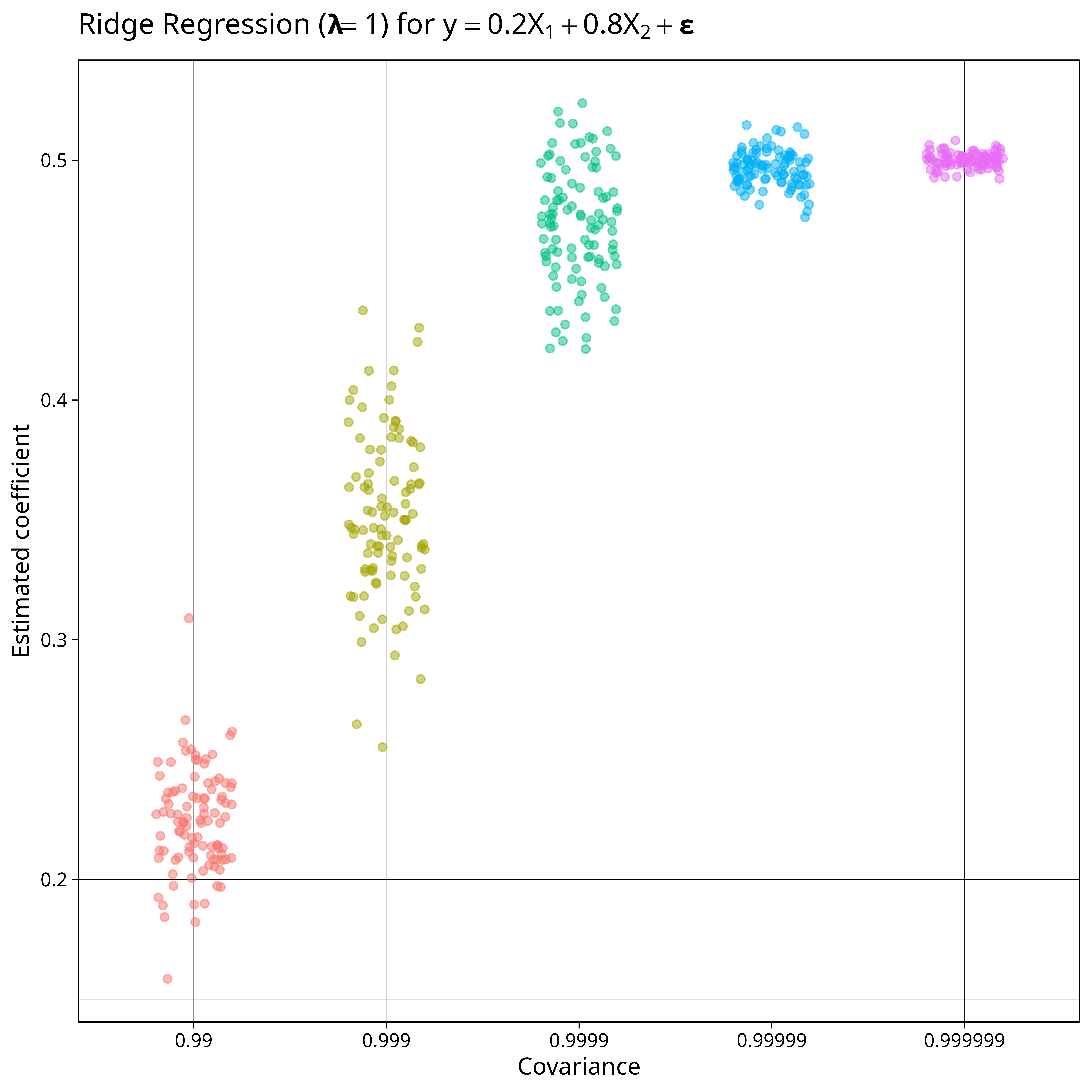
For datasets with lower multicollinearity we’re able to adjust our belief closer to the true value of \(\alpha = 0.2\) but when covariance is high, the only thing we know is that \(\alpha + \beta = 1\) and since we applied our zero-centred prior to both \(\alpha\) and \(\beta\) our model knows that \(\alpha\) and \(\beta\) aren’t 0 and sees it most likely that \(\alpha\) and \(\beta\) are both 0.5.

The MAP for a prior of \( \mathcal{N}(\mathbf{\mu}, \lambda^{-1} I) \) is \( (X^\top X + \lambda I)^{-1}(X^\top y + \mu) \). Using a prior centred around \(\alpha = 0.2\) gives us the following result

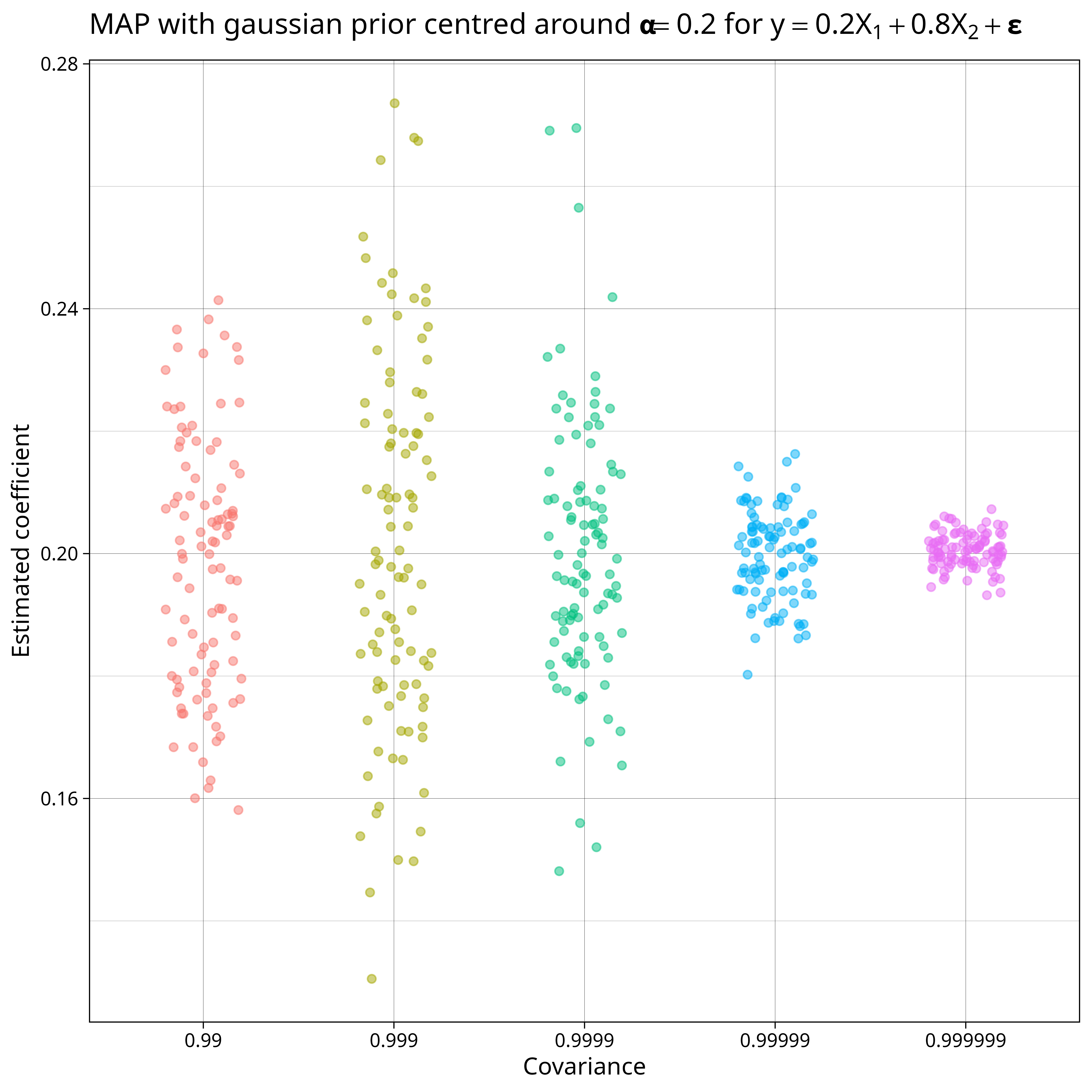
Because our highly correlated predictors are such weak evidence for any value, our MAP stays close to our prior belief of 0.2.

It would be “more Bayesian” to skip the MAP point estimate and just calculate the posterior distribution using MCMC but I would prefer to do this with PyMC in Python rather than R.

That’s for another day!

References

[1]: Murphy, Kevin P. Probabilistic machine learning: an introduction. MIT press, 2022.