What is a good Brier score? - Looking at implied probabilities from Manifold Markets

Let’s say I ask you “will it rain tomorrow?” and you respond “it will probably rain tomorrow”, what does “probably” mean?

One interpretation of this is that when we consider all possible future worlds, it rains more often than it doesn’t but this might not make all that much sense as we’re only able to experience one of these worlds.

Another way that we can think about this in terms of games or bets. Imagine that I’m going to flip a coin ten times, and I will pay you one unit of my preferred currency, the Pound sterling, every time it turns up heads. How much would you pay to play this game? The expected value from playing this game is £5 since you would expect the coin to turn up heads roughly half the time.

We can transform the question of whether it will rain tomorrow into a game like this. I’ll pay you £1 if it rains tomorrow and otherwise I will pay you nothing. How much would you pay to play this game? The fact that you think that it’s more likely to rain than not implies that you’d expect your payout to be closer to £1 than it is to £0. In other words, you’d value this game more than 50p.

Now that we have this game, we can evaluate how good your predictions are by evaluating how much money you’re making or losing in the long run. If you’re losing money then you’re consistently overstating the chances of an event occurring. If, on the other hand, you’re making large sums of money in the long run then you’re understating the chances of an event occuring.

Manifold Markets is a website that hosts several user-created games like this called “markets” using play-money called Mana. Users can pose questions such as Will Ding Liren win the 2024 World Chess Championship? and put Mana on the outcome of events.

Another way you could evaluate predictions is by assigning a score to each pair of prediction and outcomes. So predicting a 20% probability for an event that happens would give you a worse score than predicting 80% for that event.

The Brier score for a series of predictions is defined as the mean squared difference between the outcome of an event and the forecast probability for the event. Where your forecast \(f_i\) is the probability you assign to the event occurring and the outcome, \(o_i\) is 0 if the event did not occurr and 1 if it did. As an equation that looks like this.

\[\text{Brier Score} = \frac{1}{N} \sum_{i=1}^N(o_i - f_i)^2\]

If I was completely uniformed about every event then intuitively I would forecast 50% for every single event as I’m indifferent between both options. And we can prove that for any symmetric distribution this is the constant function that minimises the Brier score.

If we model events whose as having an underlying true probability, \(p\), that follows some distribution and an outcome that is 1 with probability \(p\) and is 0 with probability \(1 - p\) then the expected brier score for forcasting \(c\) for everything is

\[ \int_0^1 f(p)\left((1 - p)c^2 + p(1 - c)^2\right) dp \]

If this distribution is symmetric around 0.5 then we have

\[ \begin{align*} \mathbb E \left[\text{Brier Score}\right] &= \int_0^1 f(p)\left((1 - p)c^2 + p(1 - c)^2\right) dp \\ &= \int_0^{\frac{1}{2}} f(p)\left((1 - p)c^2 + p(1 - c)^2\right) + f(1 - p)\left(pc^2 + (1 - p)(1-c)^2 \right)dp \\ &= \int_0^{\frac{1}{2}} f(p)\left((1 - p)c^2 + p(1 - c)^2\right) + f(p)\left(pc^2 + (1 - p)(1-c)^2 \right)dp \\ &= \int_0^{\frac{1}{2}} f(p)\left((1 - p)(c^2 + (1 - c)^2) + p((1 - c)^2 + c^2)\right)dp \\ &= \int_0^{\frac{1}{2}} f(p)\left(c^2 + (1 - c)^2\right)dp \\ &= \frac{c^2 + (1 - c)^2}{2} \end{align*} \]

This has a minimum of 0.25 at \(c = 0.5\) so if your Brier score is above 0.25 you are doing worse than predicting every event with 50% probability.

We might expect the distribution of “true probabilities” to be uniform or perhaps even follow a logit-normal distribution. If we make the assumption that the market price is the true probability then we can investigate this further by looking at data from markets on Manifold.

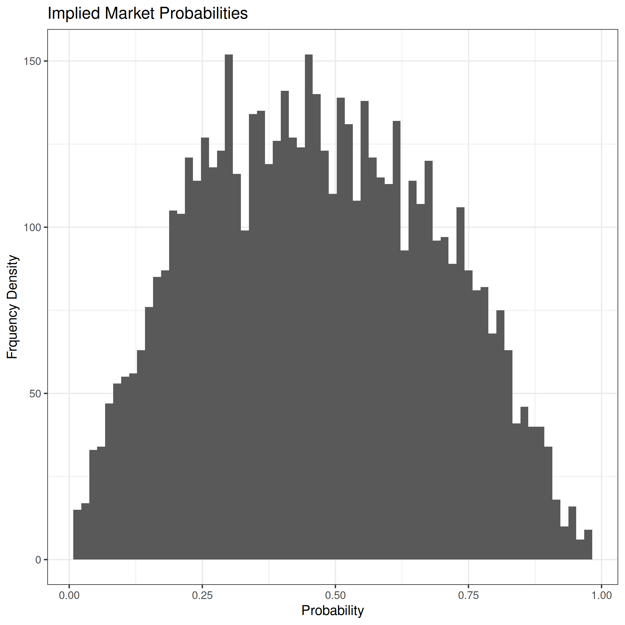
I took implied market probability data from markets on Manifold. Since I know I’m going to be taking log-odds I dropped rows where the implied probability was larger than 99% or below 1% and saw the following distribution which doesn’t look very uniform. I also dropped all rows with fewer than 50 unique bettors. The histogram for the data looks like this

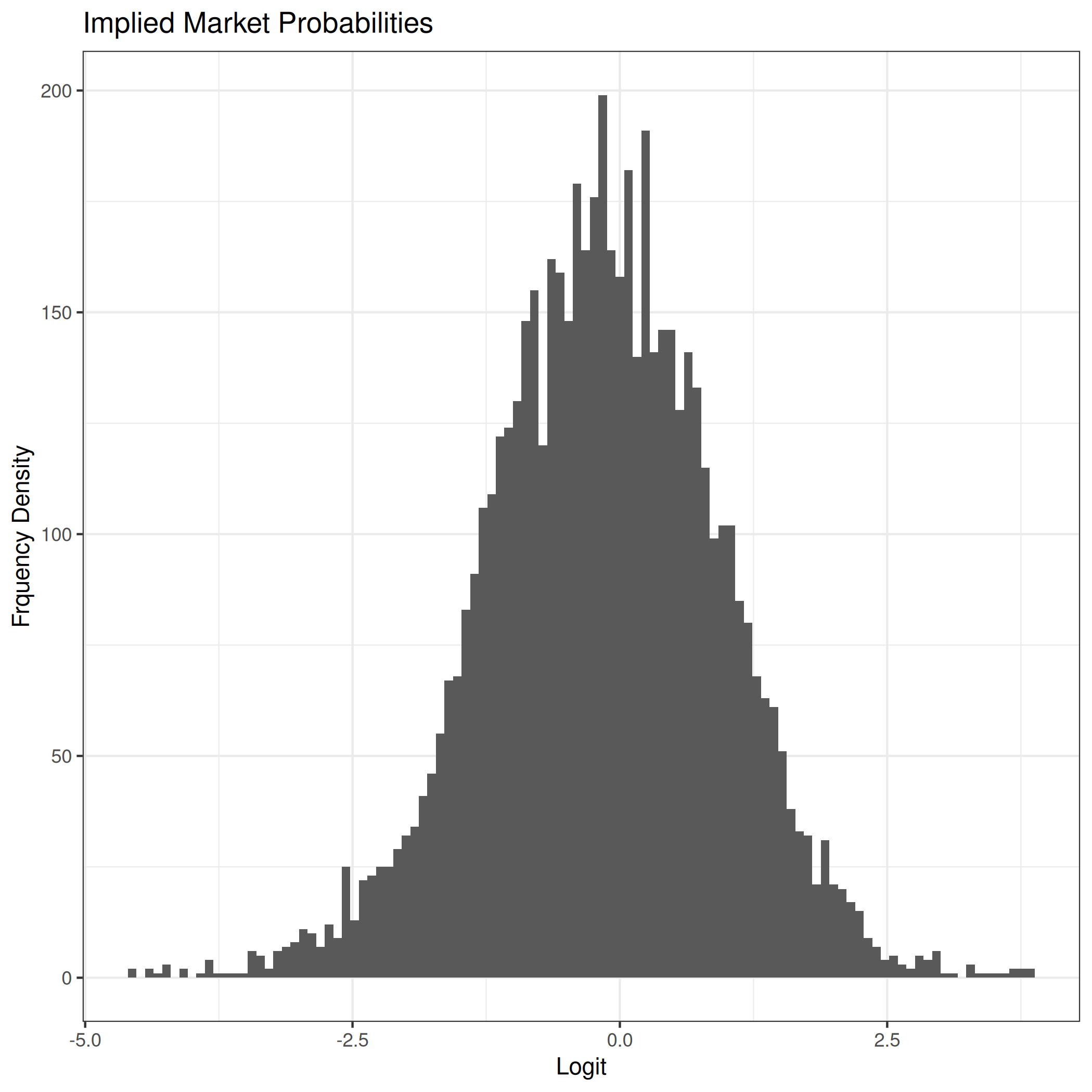
Taking logits we get the following distribution

To fit the logit-normal model I used the maximum likelihood estimators for \(\mu\) and \(\sigma\).

The pdf for the logit-normal distribution is \(f(x) = \frac{1}{\sigma \sqrt{2\pi}x(1-x)} e^{\frac{\left(\operatorname{logit}(x) - \mu\right)^2}{2\sigma^2}}\). Assuming our observations, \(X\), are independent our likelihood function looks like

\[ \mathcal{L}(\theta | X) = \prod_i^N \frac{e^{\frac{\left(\operatorname{logit}(x) - \mu\right)^2}{2\sigma^2}}}{\sigma \sqrt{2\pi}x(1-x)} \]

Taking logs we get

\[ \log \mathcal{L}(\theta | X) = \sum_{i=1}^N \log \frac{e^{\frac{\left(\operatorname{logit}(x) - \mu\right)^2}{2\sigma^2}}}{\sigma \sqrt{2\pi}x(1-x)} \]

Differentiating this with respect to \(\mu\) to find the maximum we get

\[ \begin{align*} \frac{\partial \log \mathcal{L}}{\partial \mu} &= \frac{\partial}{\partial \mu} \sum_{i=1}^N \log \frac{e^{\frac{\left(\operatorname{logit}(x) - \mu\right)^2}{2\sigma^2}}}{\sigma \sqrt{2\pi}x(1-x)} \\ &= \frac{\partial}{\partial \mu} \sum_{i=1}^N \log e^{\frac{\left(\operatorname{logit}(x) - \mu\right)^2}{2\sigma^2}} - \log \sigma \sqrt{2\pi}x(1-x) \\ &= \frac{\partial}{\partial \mu} \sum_{i=1}^N \log e^{\frac{\left(\operatorname{logit}(x) - \mu\right)^2}{2\sigma^2}} \\ &= \frac{\partial}{\partial \mu} \sum_{i=1}^N \frac{\left(\operatorname{logit}(x) - \mu\right)^2}{2\sigma^2} \\ &= \frac{1}{2\sigma^2} \frac{\partial}{\partial \mu} \sum_{i=1}^N \left(\operatorname{logit}(x) - \mu\right)^2 \\ &= \frac{1}{2\sigma^2} \sum_{i=1}^N -2\left(\operatorname{logit}(x) - \mu\right) \\ &= -\frac{1}{\sigma^2} \sum_{i=1}^N \operatorname{logit}(x) - \mu \\ &= -\frac{1}{\sigma^2} \sum_{i=1}^N \operatorname{logit}(x) - \mu \\ &= \frac{1}{\sigma^2} \left(\mu N - \sum_{i=1}^N \operatorname{logit}(x) \right)\\ &= \frac{N}{\sigma^2} \left(\mu - \frac{1}{N}\sum_{i=1}^N \operatorname{logit}(x) \right)\\ \end{align*} \]

Which has a value of 0 precisely when \(\mu\) is the sample mean of the logits of our observation. I used the same procedure to find the MLE for \(\sigma\).

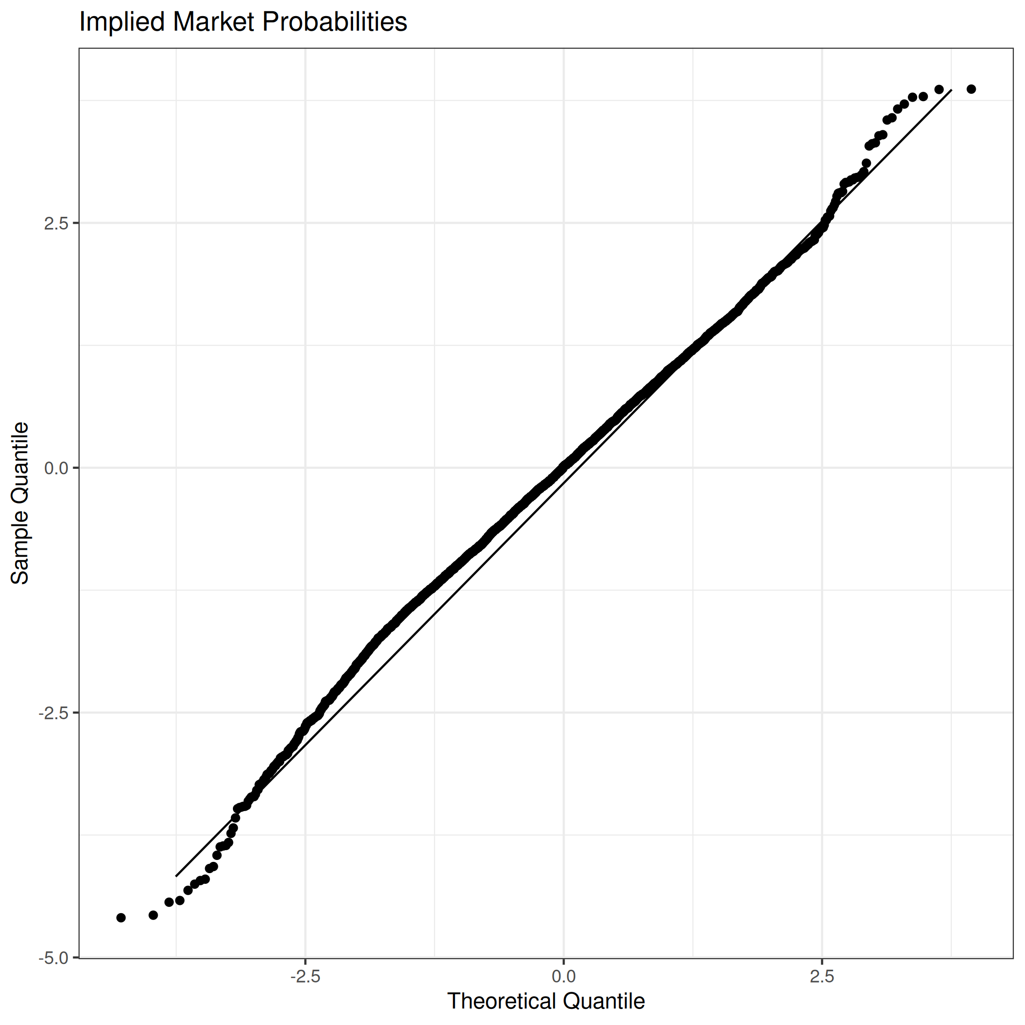
The QQ-plot looks roughly normal however the distribution is biased towards 0.

Despite this, the distribution is pretty symmetric so as discovered earlier, you should aim for a Brier score of below 0.25 (0.5 if you multiply by 2 like Fatebook) or else you’re uncalibrated. The true mean is actually \(0.47\) so you scould achieve a slightly better brier score by always guessing slightly below 50%.