Benchmarking my perception of sound
15 December 2024
Learning about Bayesian statistics and the Jeffreys prior
I’ve been learning about Bayesian statistics and computational methods recently so I want to work on a few small projects to put into practice what I have been learning.
Today I decided to benchmark my perception of sound: I created a game where I’m played a random tone and I have to respond with a number that is as close as possible to the frequency that was played. I sample frequencies uniformly at random between 131Hz and 495Hz.
I wanted to do this experiment as I came up for two models for how I’d perform on this game. If we let \(Y\) be the frequency I report and \(X\) be the frequency that I actually heard, my first model is that I will give the frequency that I heard added to some normally distributed error term, that is
\[Y_i = X_i + \epsilon_i \]
Where \(\epsilon_i \sim \mathcal{N}(\mu, \sigma^2)\). If this is the case, I’d expect \(\mu\) to be zero as I don’t expect to have a consistent bias to guessing higher or lower than the actual frequency.
My second model is motivated by the fact that human sound perception is inherently logarithmic and musical intervals are actually frequency ratios. For example, playing C3 then E3 sounds the same as playing a C4 then E4: it’s just an octave higher however the difference between C3 and E3 is about 35Hz and the difference between C4 and E4 is about 70Hz. And in fact, an octave difference is a doubling of the frequency not a fixed difference in Hz. My second model hypothesises that the differences between the logarithms of the frequencies or “cents” is normally distributed.
\[ \log Y_i = \log X_i + \epsilon_i \]
Where \(\epsilon_i\) is again a normally distributed error term.
I decided to test these two models as I hypothesised that my absolute error in frequency would become worse for higher tones which is a consequence of the second model but not the first model. This came about as earlier this week, I began teaching myself to report numerical frequencies as opposed to the musical note names: I wanted to teach myself to respond with “440 Hertz” as opposed to “A4” in response to hearing a tone played at 440Hz.
I quickly created a python script to collect this data. It looks like this
import pysine
import random

LOWEST = 131
HIGHEST = 494
should_continue = True
played = []
heard = []
iteration = 0
try:
    while should_continue:
        iteration += 1
        tone = LOWEST + random.random() * (HIGHEST - LOWEST)
        read = None
        while read is None:
            pysine.sine(tone)
            entered = input(f"{iteration}>> ").lower().strip()
            if entered == "q":
                should_continue = False
                break
            if entered == "r":
                continue
            try:
                read = float(entered)
            except:
                print("Unable to read number")
        print(f"Played {tone}, you heard {read}")
        played.append(tone)
        heard.append(read)
except KeyboardInterrupt:
    pass
except EOFError:
    pass

print("tone,heard")
for x, y in zip(played, heard):
    print(f"{x},{y}")
Here are the results from my first play through of the game where I answered 20 questions
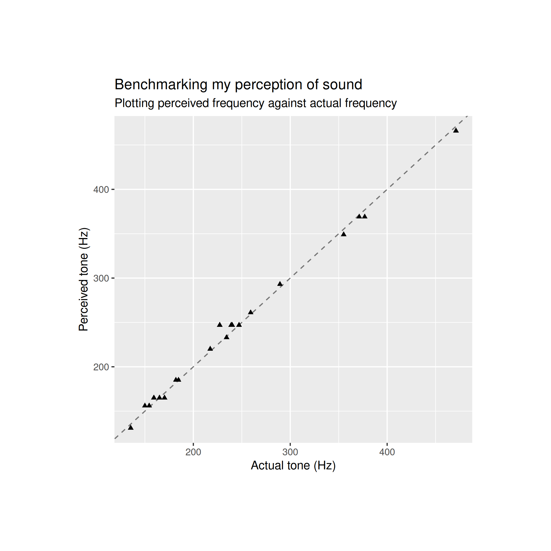
From a glance both of these models seem fairly sensible: my reported frequency appears to closely track the frequency that I actually heard. The error plot for my first game looks like this
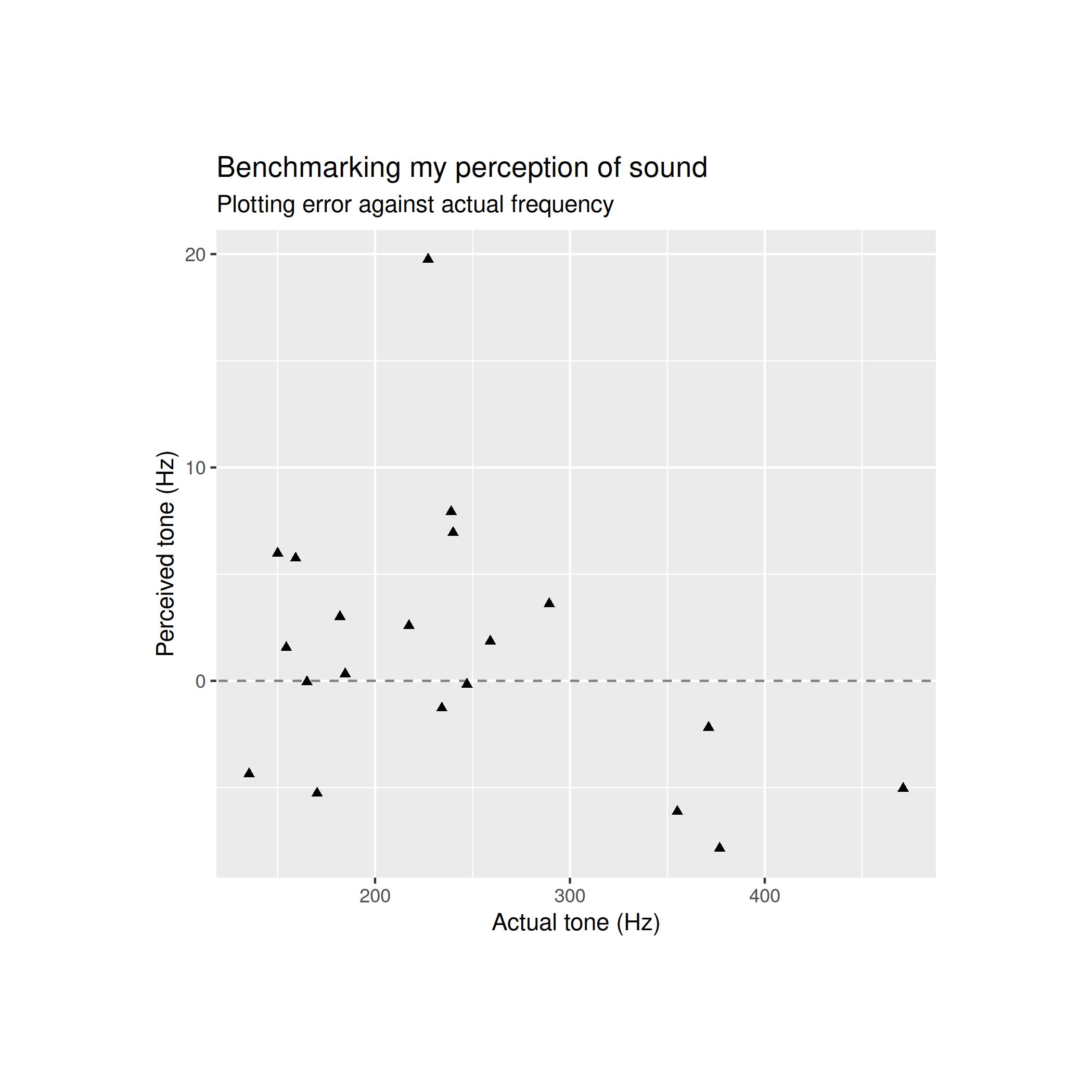
It’s hard to get any insights from this by just analysing the data visually, so I turn to statistics to compare how well these models explain the data.
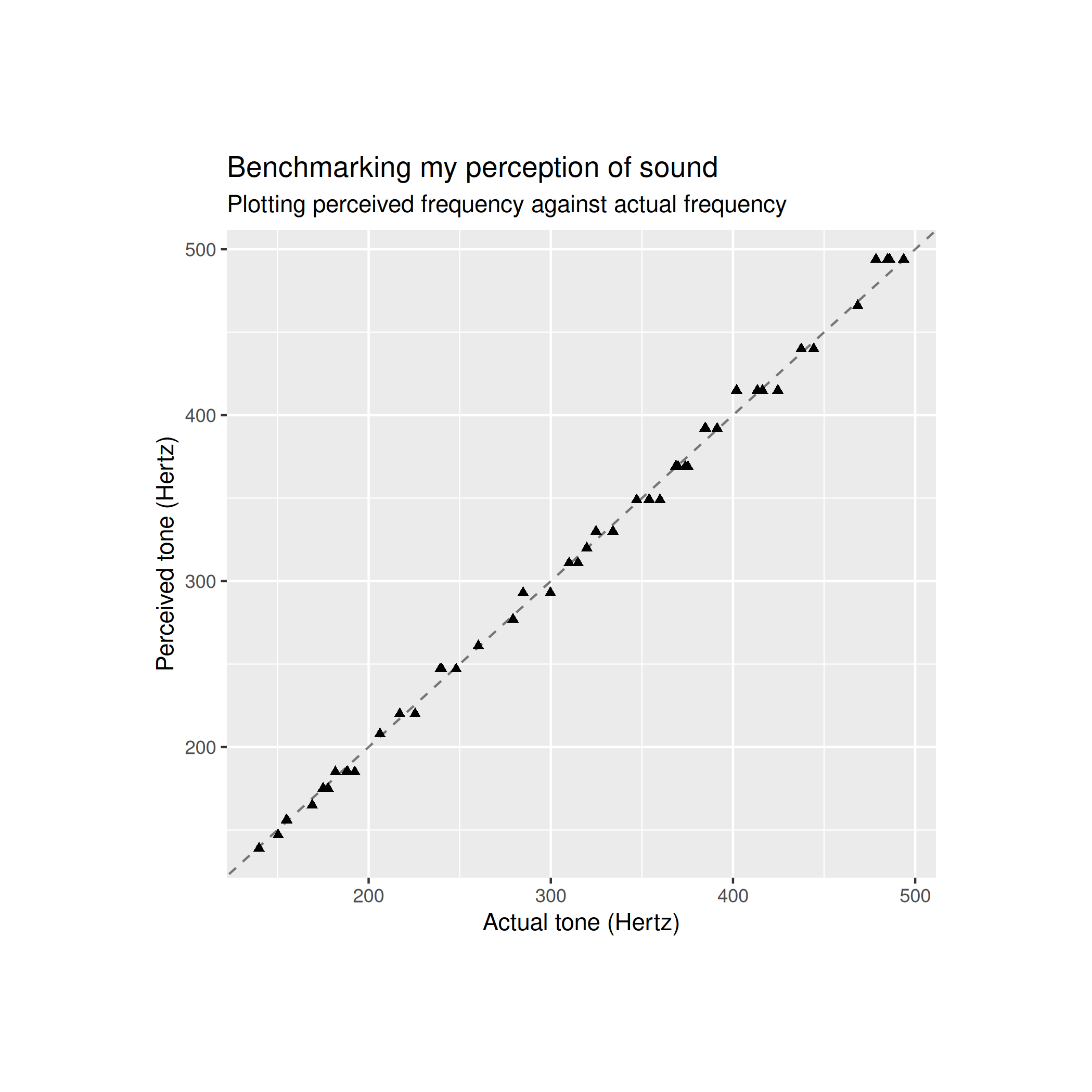
The first thing I do is play another round of the game but this time I listen to 50 tones instead of just 20. The sine waves were also pretty boring to listen to so I synthesised my own instrument however I did a quick runthrough of the game with the synthesiser I made and I noticed that there was a clear upwards bias in the frequency that I reported. I reverted back to using sine waves and noticed that this bias disappeared which indicates that this bias was an artefact of how I wrote my synthesiser. I added harmonics but not subharmonics to my synth so this may have caused me to perceive the notes from the synthesiser as being higher than they actually were. That’s the euphemistic way of explaining that I wrote a bad synth.
After going back to using sine waves, the data I’m analysing looks like this
The error looks like this
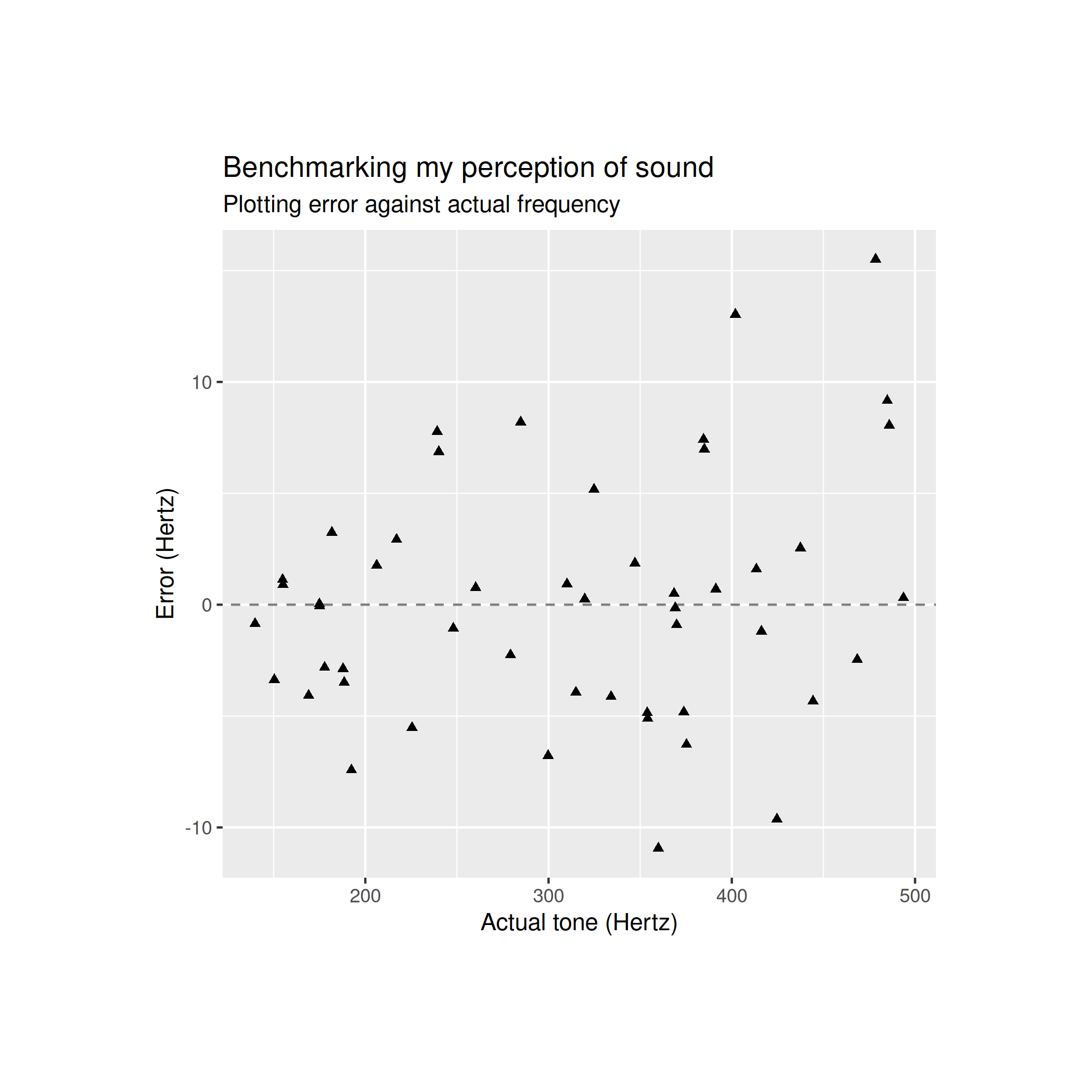
Now, the absolute error looks like this
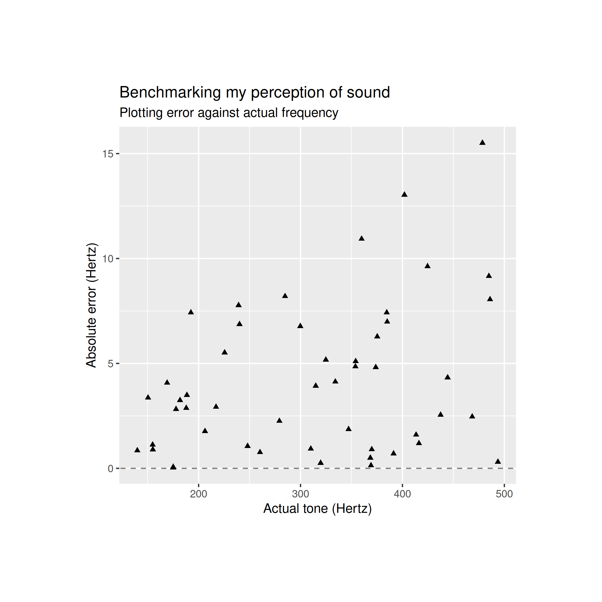
This final graph is important as it shows that the error term is clearly heteroskedastic which means that the variance of the error term is not constant: the error term has much larger variance for higher frequencies.
This matters because the first model predicts a homoskedastic resdiual term which does not match the data. My second model predicts heteroskedasticity but also predicts that the error for log frequency is homoskedastic. The plot for the absolute error between log frequencies looks like this
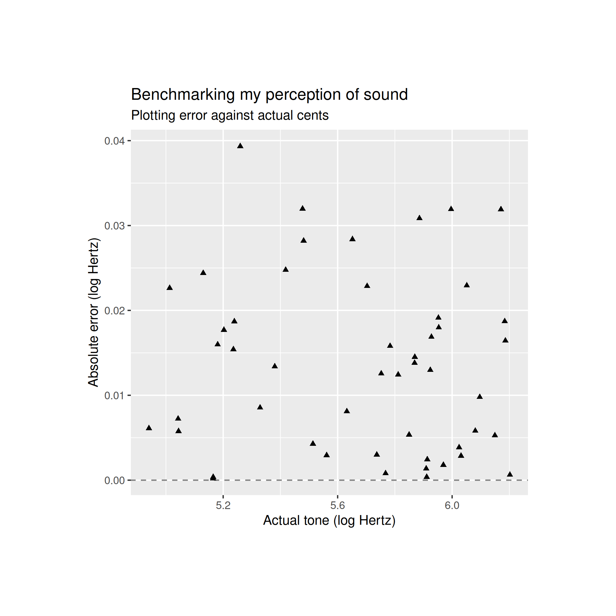
Visually, this is homoskedastic which is really good for the second model and is strong evidence that the second model better explains the data. Now, let’s quantitatively examine these models using bayesian statistics.
Bayesian statistics centres itself around Bayes’ rule which states that \(p(\theta | x) \propto p(x | \theta) \times p(\theta) \) or that the likelihood of \(\theta\) after having observed \(x\) is proportional to the prior likelihood of theta multiplied by the probability of observing \(x\) with parameter \(\theta\).
What does this mean? If we have a distribution representing our beliefs about the value of \(\theta\), Bayes’ rule tells us how to update our beliefs after observing new data. The distribution from before observing the data is called our “prior” and the updated distirbution after observing the data is called the “posterior”.
If we fix \(\mu = 0\) for both models then both models become single paramter models as we have \(\epsilon_i \sim \mathcal{N}(0, \sigma^2)\). What is my prior distribution for \(\sigma\)?
For the sake of learning I’d like to use an uninformative prior: specifically, the Jeffreys prior, named after Harold Jeffreys.
The Jeffreys prior gives us a prior distribution that is invariant under montone transformations of the parameter. For example, if I took a uniform distribution as my prior for \(\sigma^2\) between 0 and 1 then the implied distribution of \(\sigma\) would also be between 0 and 1 but it would not be uniform. We can contrast this to the Jeffreys prior where the Jeffreys prior for \(\sigma^2\) aligns with the Jeffreys prior for \(\sigma\).
The Jeffrey’s prior is specified as proportional to the square root of the determinant of the Fisher information matrix.
\[ p(\theta) \propto \sqrt{\operatorname{det} \mathcal{I}(\theta)} \]
Our normal distribution with mean 0 looks like
\[ f(x ; \sigma) = \frac{1}{\sqrt{2\pi\sigma^2}} e^{-\frac{x^2}{2\sigma^2}} \]
We have a single parameter model so we get
\[ \begin{align*} p(\sigma) &\propto \sqrt{\mathbb E \left[ \left. \left( \frac{\partial}{\partial \sigma} \log f(x;\sigma) \right)^2 \right| \sigma \right]} \\ &= \sqrt{\mathbb E \left[ \left( \frac{\partial}{\partial \sigma} \log \frac{1}{\sqrt{2\pi\sigma^2}} e^{-\frac{x^2}{2\sigma^2}} \right)^2 \right]} \\ &= \sqrt{\mathbb E \left[ \left( \frac{\partial}{\partial \sigma} \log e^{-\frac{x^2}{2\sigma^2}} - \log \sqrt{2\pi\sigma^2} \right)^2 \right]} \\ &= \sqrt{\mathbb E \left[ \left( \frac{\partial}{\partial \sigma} - \frac{x^2}{2\sigma^2} - \log \sigma - \frac{1}{2} \log 2\pi \right)^2 \right]} \\ &= \sqrt{\mathbb E \left[ \left( \frac{\partial}{\partial \sigma} -\frac{x^2}{2\sigma^2} - \log \sigma \right)^2 \right]} \\ &= \sqrt{\mathbb E \left[\left( \frac{x^2}{\sigma^{3}} - \frac{1}{\sigma} \right)^2 \right]} \\ &= \sqrt{\frac{1}{\sigma^2} \mathbb E \left[\left( \frac{x^2}{\sigma^2} - 1 \right)^2 \right] } \\ &\propto \sqrt{\frac{1}{\sigma^2} } \\ &= \frac{1}{\sigma} \end{align*} \]
Unfortunately, this is an improper prior and the integral across the support is not finite and does not form a true probability distribution. I’m too scared to use an improper prior after reading about how they can lead to nonsense inference results. Analysing whether or not they’re appropriate to use appears to be very complicated so I’ll stay away from improper priors for a few years.
Fortunately, I can create my own uninformative prior. I want to feign ignorance about both the variance and the standard deviation so I’d like a prior that ensures me transformational invariance between \(\sigma\) and \(\sigma^2\) I can get this with any pair of distributions \(f_{\sigma}\) and \(f_{\sigma^2}\) that satisfy
\[ \begin{align*} f_{\sigma}(x) &= \frac{dx^2}{dx} f_{\sigma^2}(x) \\ &= 2xf_{\sigma^2}(x) \end{align*} \]
So we now have
\[ \begin{align*} \int_a^{\infty} f_{\sigma^2}(x) dx &= \int_a^\infty f_{\sigma}(x) dx \\ \int_a^{\infty} f_{\sigma^2}(x) dx &= \int_a^\infty 2xf_{\sigma^2}(x) dx \\ \int_a^{\infty} f_{\sigma^2}(x) \left( 1 - 2x \right) dx &= 0 \end{align*} \]
Integrating this by parts we get
\[ \begin{align*} \int_a^{\infty} f_{\sigma^2}(x) \left( 1 - 2x \right) dx &= 0 \\ -f_{\sigma^2}(0) + 2 \int_a^\infty F_{\sigma^2}(x) dx &= 0 \\ 2 \int_a^\infty F_{\sigma^2}(x) dx &= f_{\sigma^2}(a) \\ 2 \mathbb E\left[\sigma^2\right] dx &= f_{\sigma^2}(a) \end{align*} \]
Where \(F_{\sigma^2}\) denotes the CDF for \(f_{\sigma^2}\) and \(a\) lower bounds the variance in this distribution. Unfortunately, I do not want to solve this functional equation so I’ll just use the Jeffreys prior.
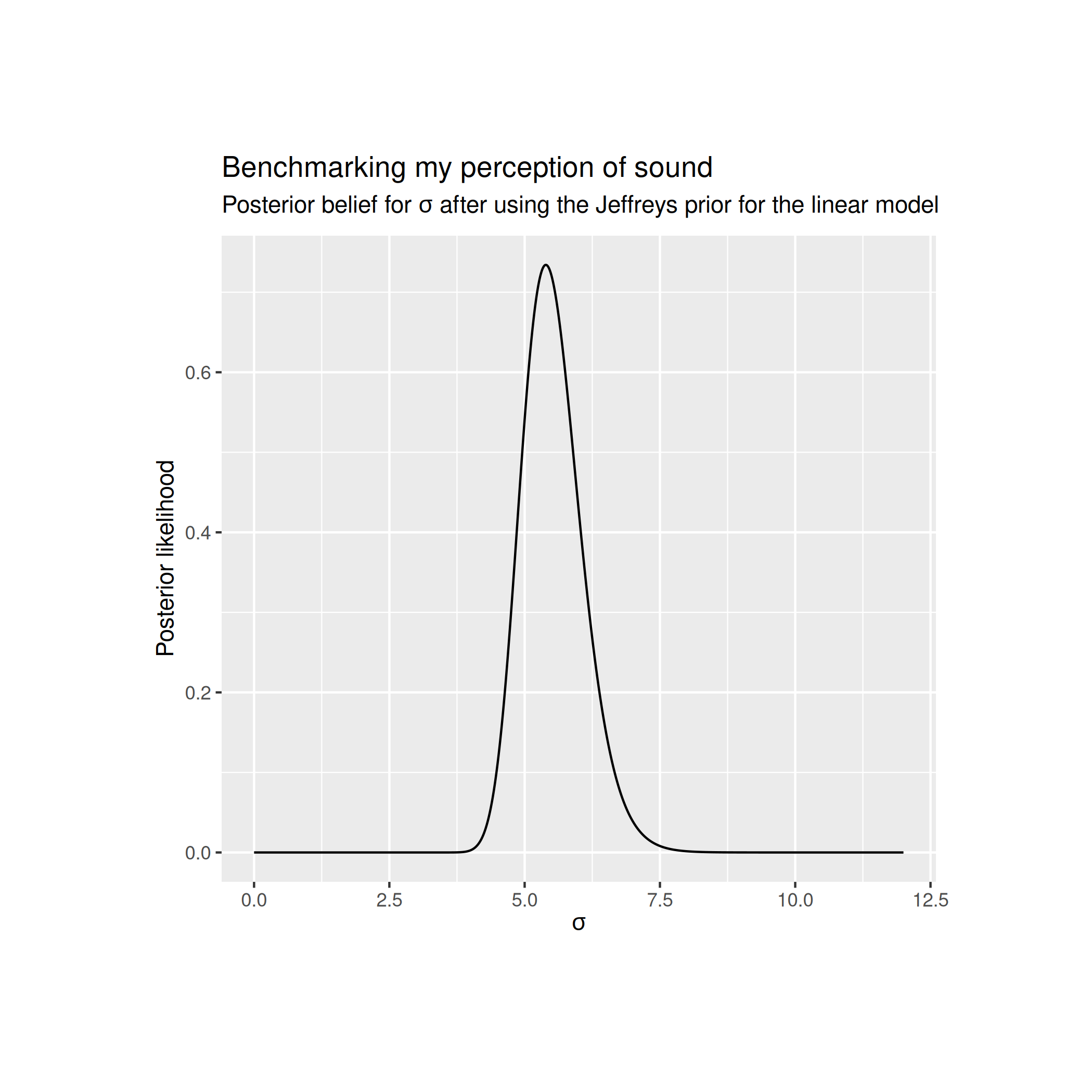
Using the Jeffreys prior for the linear model gives me the following posterior distribution
The Jeffreys prior for the log-linear model gives me the following posterior distribution
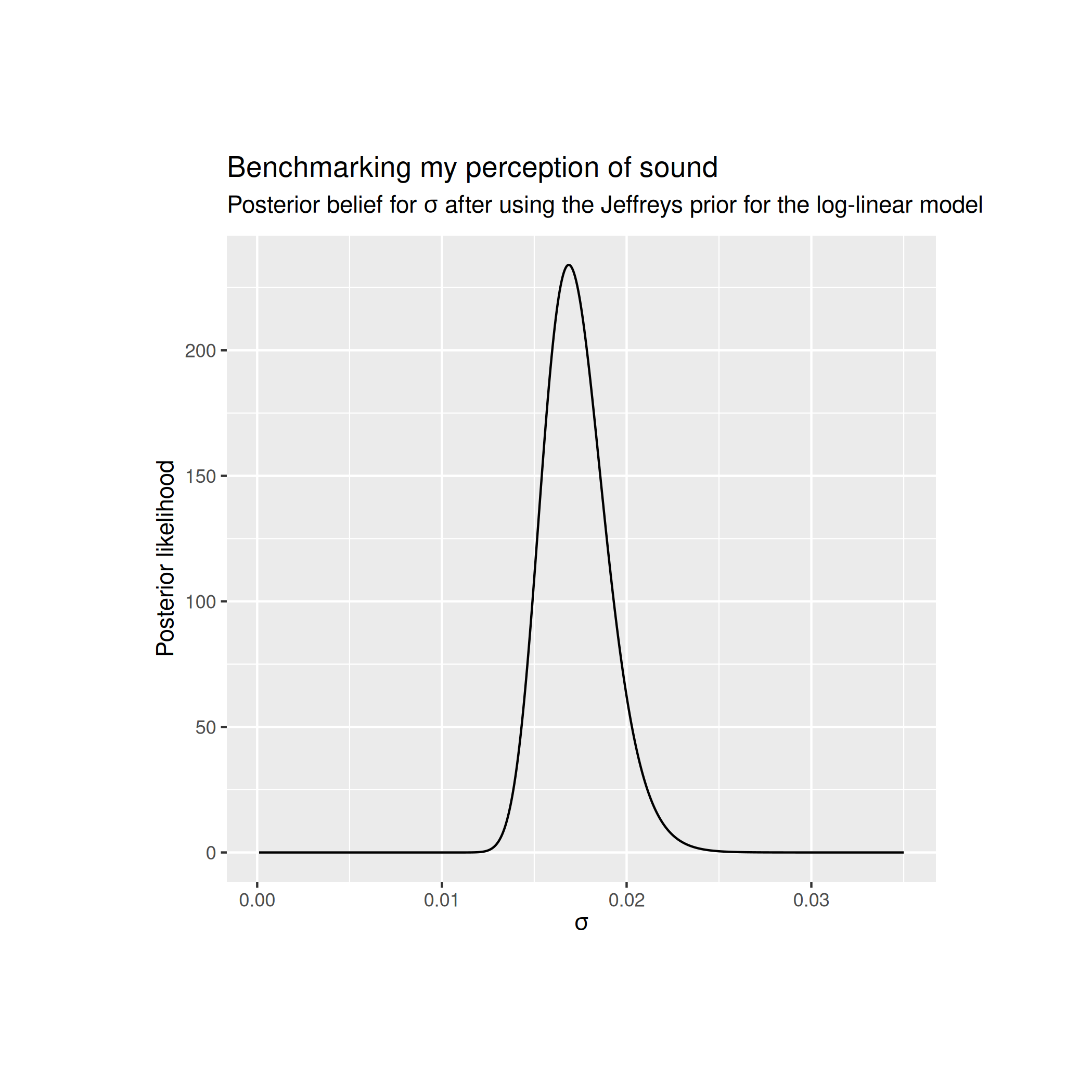
After taking the MLE for each of these models I can find a point estimate for the Bayes factor for the two models. The Bayes factor allows me to quantify how much better one model explains the data than another.
My code for calculating the likelihoods for each of the models looks like this
likelihood_linear <- prod(dnorm(df$heard - df$tone, mean=0, sd=sigma_linear))
likelihood_log <- prod(dnorm(log(df$heard) - log(df$tone), mean=0, sd=sigma_log))
likelihood_log / likelihood_linear
The likelihood for the the first model is about \(10^{-68}\) whereas the likelihood for the second model comes out to be around \(10^{59}\). This gives us a ratio of about \(10^{125}\) and numerically integrating over the posterior distributions to approximate the true Bayes factor gives me about the same result which is a decisive victory for the log-linear model.
I learned a lot through this project and I really enjoyed surveying Bayesian statistics while doing background reading and was super fun all around.