The heat equation and numerical stability

Status: WIP. I want to write about implicit schemes and Gauss-Seidel. I also want to introduce Gershgorin’s circle theorem for bounding the eigenvalues of a matrix and applying this to stability analysis

1 July 2026

The heat equation, intuitively

The heat equation describes how the distribution of heat evolves in a system over time. Intuitively, we can think of the evolution of heat as a local phenomenon where we can determine how the heat changes at a point by looking at the heat in the immediate surrounding of this point.

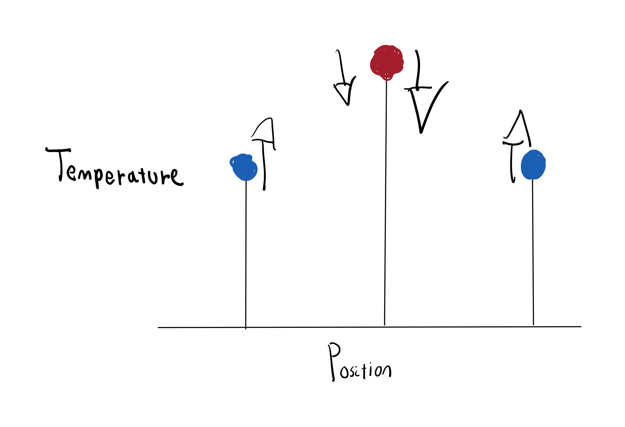
As an example we could imagine it’s June 2026 in the United Kingdom during an unexpected and very annoying heatwave and you’re in a house that’s cool on the inside but it’s 35°C outside. Suppose we open up the door, then we only need to look at the air immediately outside the house in order to work out how the heat at the door changes.

In this situation, the heat from outside enters the house which results in the warm outside air becoming slightly colder and the cool inside air becoming warmer. In general, we have the property that heat at a point tends towards the heat of its neighbours and this is one instance of the second law of thermodynamics.

This is described by the following low-budget (no-budget?) illustration where there’s cooling pressure on the hot portion of the image and heating pressure on the cool portions of the image.

As an equation we can think of this in terms of differences between the heat at neighbouring points. Let’s say we live in a discretised world where at every point \(x_i\) we have two immediate neighbours: \(x_{i - 1}\) to the left and \(x_{i + 1}\) to the right.

Let’s also imagine that time is discretised in this world so we have the heat at time \(t\) at a certain point \(i\) as \(u^{(t)}_i\) and the heat in the next time period being \(u^{(t + 1)}_i\). The question we want to answer is how heat evolves at a certain point over time, so we want to find \(u^{t + 1}_i\) given \(u^{t}_i\).

Earlier we said that a position gets warmer when it is colder than its neighbours. If we first look at the difference between the heat at position \(i\) and its neighbour on the left \(i - 1\) we get this as an expression \(u^{(t)}_i - u^{(t)}_{i - 1}\)

When the position is hotter than its left neighbour and \(u^{(t)}_i > u^{(t)}_{i - 1}\), this quantity is positive, and the change in heat at this position should be negative. When this position is cooler than its neighbour then this quantity is negative and the change in heat should be positive.

We have a similar situation for the right neighbour. That is, when the quantity \(u^{(t)}_i - u^{(t)}_{i + 1}\) is positive then this position is hotter than the right neighbour and temperature decreases. When it’s negative, the temperature increases.

If we have this change in temperature to be linear in these amounts then we get the expression for the temperature in the next state as \( u^{(t + 1)}_i = u^{(t)}_i + \kappa \left( \left( u^{(t)}_{i + 1} - u^{(t)}_i \right) - \left(u^{(t)}_i - u^{(t)}_{i-1} \right) \right)\) which we can notice as a second order difference, a difference of differences. This is unrelated to differences in differences from econometrics.

If we have the grid described by a continuous function and our grid is sufficiently fine then in the limit this second order difference becomes a second order spatial derivative, which we can denote as \(\frac{\partial^2 u}{\partial x^2} = \nabla^2 u = \triangle u\). Replacing our equation with a derivative gets us \( u^{(t + 1)}_i = u^{(t)}_i + \kappa \frac{\partial^2 u}{\partial x^2}\).

In the limit of our time steps becoming more fine, we similarly get the temporal difference becoming a derivative with respect to time which allows us to write our expression for the change in heat as

\[ \frac{\partial u}{\partial t} = \kappa\triangle u \]

Which gives us the heat equation. We also have an alternative derivation using conservation of energy.

We can extend this model so that we can consider how heat diffuses over a 2 dimensional grid instead of a line of points. The details remain largely the same and this equation generalises to higher dimensions.

Solving the heat equation numerically

Often, we don’t know the spatial derivative, so when writing programs we stick to the discretised form of the equation where we use the finite difference formulation from earlier.

\[ u^{(t + 1)}_i = u^{(t)}_i + \kappa \left( \left( u^{(t)}_{i + 1} - u^{(t)}_i \right) - \left(u^{(t)}_i - u^{(t)}_{i-1} \right) \right)\]

This has the obvious code implementation where we iterate over all of our points in the grid, calculate the second differences then use our equation for \(u^{(t + 1)}_i\). This algorithm is called explicit euler and it falls under a class of algorithms called “time stepping schemes”. Since we’re finding values of \(u^{(t)}_i\) by effectively stepping through time.

This scheme works but is unstable when our grid is too fine or high-res, or our timesteps are too big. If we want this scheme to be stable (we do), then the precise statement is that we need to have \(\frac{\kappa \Delta t}{\Delta x^2} \leq \frac{1}{2} \) where \(\Delta t\) corresponds to the size of our steps through time and \(\Delta x\) corresponds to how far apart our grid points are.

I’m going to walk through how we can show this statement, it’s similar in nature to the CFL condition which also gives bounds on the timestep size and grid discretisation required for stabiltiy.

We can create a vector \(u^{(t)}\) that represents the temperature \(u^{(t)}_i\) at a certain point in time, \(t\). Our formula for calculating \(u^{(t+1)}\) from \(u^{(t)}\) is linear in the entries of \(u^{(t)}\) so we have a matrix \(A\) that describes the transformation from the old timestep to the new timestep. We can write this as

\[u^{(t+1)} = Au^{(t)}\]

We can iterate this linear transformation to get the heat at an arbitrary point in time, which gives us an expression in terms of the matrix power \(A^n\)

\[u^{(n)} = A^n u^{(0)}\]

Floating point error and numerical stability

Since computers are finite and we don’t have infinite precision maths, we use floating point numbers as approximations for the real numbers. So instead of storing \(\pi\), we store a finite approximation of pi. In C, the M_PI macro is defined as 3.14159265358979323846.

Floating point also approximates most rational numbers and you can notice this when we try to evaluate \(0.1 + 0.2\) which gives us 0.30000000000000004 in Python.

The reason for this is that we can’t store any of \(\frac{1}{10}\), \(\frac{2}{10}\) or \(\frac{3}{10}\) exactly in floating point, this means we need to round them to the nearest representable number. Because of this, we incur numerical error after every floating point operation and for the specific case of 0.1 + 0.2 this error becomes noticeable enough that we can see the error after not so many significant digits.

We can see the floating point error associated with storing each number in Python by printing each number with high-precision

>>> print(f"{0.1:.55f}")
0.1000000000000000055511151231257827021181583404541015625
>>> print(f"{0.2:.55f}")
0.2000000000000000111022302462515654042363166809082031250
>>> print(f"{0.3:.55f}")
0.2999999999999999888977697537484345957636833190917968750
>>>

You can notice that none of the printed values are the same as the exact values. The name for the difference between the computed result and the actual result is called roundoff error and we can analyse the effect of floating-point roundouff error on the stability of our timestepping scheme.

Let’s suppose that our initial condition \(u^{(0)}\) is stored exactly, then we can look at the difference in the results from our algorithm when using actual numbers and the result that we get when using floating point numbers.

Let’s use \(v^{(t)}\) to denote the result of running our algorithm using an idealised, infinite precision arithmetic.

Our error \(\epsilon^{(t)}_i\) is now \(\epsilon_t = v^{(t)} - u^{(t)}\). We can rewrite \(v^{(t)}\) using the definition of our algorithm

\[ \begin{align*} v^{(t + 1)}_i &= v^{(t)}_i + \kappa \left( \left( v^{(t)}_{i + 1} - v^{(t)}_i \right) - \left(v^{(t)}_i - v^{(t)}_{i-1} \right) \right) \\ Av^{(t)} &= Av^{(t + 1)} \end{align*} \]

We can also take into account floating point error that comes from the imprecision from our maths. So instead of having \(u^{(t + 1)} = Au^({t})\) we now have \(u^{(t+1)} = Au^({t}) + \eta^{(t + 1)}\)

Using this, our error at time \(t + 1\) becomes the following

\[ \begin{align*} \epsilon^{(t+1)} &= v^{(t + 1)}_i - u^{(t + 1)}_i \\ \epsilon^{(t+1)} &= Av^{(t)}_i - \left(Au^{(t)}_i + \eta^{(t + 1)}\right) \\ \epsilon^{(t+1)} &= A\left(v^{(t)}_i - u^{(t)}_i\right) - \eta^{(t + 1)} \\ \epsilon^{(t+1)} &= A\epsilon^{(t)} - \eta^{(t + 1)} \\ \end{align*} \]

And we have the result that the error follows a recurrence relation very similar to the recurrence relation our algorithm implements. If the initial condition is stored precisely and \(\epsilon^{(0)} = 0\) then we get the following expression for theerror at time \(t\)

\[\epsilon^{(t)}=-\sum_{k=1}^{t}A^{t-k}\eta^{(k)}\]

We can bound the size of this error using the inequality \(|Av| \leq |A||v| \), where \(|\cdot|\) is a matrix norm which quantifies the largest amount a matrix scales a vector. Once we do that, we get the following

\[ \begin{align*} \left|\epsilon^{(t)}\right|\le\sum_{k=1}^{t}\left|A\right|^{t-k}\left|\eta^{(k)}\right| \end{align*} \]

If our one-step floating point errors are bouded by \(\eta_{\max}\) then we get the following

\[ \begin{align*} \left|\epsilon^{(t)}\right| &\le \eta_{\max}\sum_{k=0}^{t-1}\left|A\right|^k \\ \end{align*} \]

One thing to note is that this is the sum of a geometric series and if \(|A| \geq 1\) then this bound diverges exponentially as we increase \(t\). If \(|A| < 1\) then \(|A|^t\) decays exponentially and our error grows only linearly over time, which we see after the following simpliciation

\[ \begin{align*} \left|\epsilon^{(t)}\right| &\le \eta_{\max}\sum_{k=0}^{t-1}\left|A\right|^k \\ &\le \eta_{\max}\sum_{k=0}^{t-1} 1^k\\ &\le t\eta_{\max} \end{align*} \]

For this reason we can call our scheme stable if \(|A| < 1\) and unstable otherwise.

That being said, it’s not really clear what \(|A|\) is or how we find this out. We haven’t even explicitly defined \(A\) yet or what the matrix norm \(|\cdot|\) is.

Earlier I mentioned that the matrix norm measures the largest amount that the matrix scales a vector by. We can be more precise and say that we’re looking at the ratio between the magnitude of a vector and the result after multiplying by \(A\). So we have that as \(|A| = \max_x \frac{|Ax|}{|x|}\).

Since we want to find the value of \(|A|\), it helps to know what \(A\) is. If we think about \(A\) in terms of a linear map going from our old 1-dimensional grid to the 1-dimensional grid in the new timestep, then each row of \(A\) corresponds to a point in the new 1-dimensional grid and the entries in this row describe the linear combination of the points in the old 1-dimensional grid.

Since each point in the new grid only depends on three values from the old grid (the point itself, its left neighbout and its right neighbour) every row in our matrix corresponds to 3 values.

Technically the boundaries only use 2 values and if we were being more rigorous about this, we could explicitly use a scheme to fill in the values for their missing neighbours. Of these schemes, we have the Dirichlet scheme which sets them to zero and the Neumann scheme which sets them the same value as their neighbour.

Earlier we established that the equation for the value of a point in the new timestep has the following form \[u^{(t + 1)}_i = u^{(t)}_i + \kappa \left( \left( u^{(t)}_{i + 1} - u^{(t)}_i \right) - \left(u^{(t)}_i - u^{(t)}_{i-1} \right) \right)\]

We can rewrite this as an explicit linear combination of the values at the neighbouring points

\[u^{(t + 1)}_i = \kappa u^{(t)}_{i-1} + (1 - 2\kappa) u^{(t)}_i + \kappa u^{(t)}_{i+1}\]

This makes it clearer what the strucure of the matrix \(A\) is. When thinking about matrices as linear operations described with respect to a fixed basis, each row represents an output and each column represents an input. Our matrix \(A\) has \(n\) inputs which represent the points in the old timestep, and \(n\) outputs which represent the points in the new timestep. This means \(A\) is an \(n \times n\) matrix.

The values in each of the rows describe the coefficients of the linear combination corresponding to each output. So since the \(u^{(t + 1)}_i\) has coefficients \(1\), \(1 - 2\kappa\) and \(1\) corresponding to positions \(i - 1\), \(i\), and \(i + 1\) respectively, row \(i\) will have entries \(1\), \(1 - 2\kappa\) and \(1\) in columns \(i - 1\), \(i\), \(i + 1\).

More explicitly, the matrix looks like the following

\[ A = \begin{bmatrix} 1 - 2\kappa & \kappa & 0 & \cdots & 0 \\ \kappa & 1 - 2\kappa & \kappa & \cdots & 0 \\ 0 & \kappa & 1 - 2\kappa & \cdots & 0 \\ \vdots & \vdots & \vdots & \ddots & \vdots \\ 0 & 0 & 0 & \cdots & 1 - 2\kappa \end{bmatrix} \]

We want to find the matrix norm \(|A|\) which we defined earlier as being the largest amount that a vector is scaled by, and we wrote that as \[|A| = \max_x \frac{|Ax|}{|x|}\]

We can simplify this a bit by only considering unit vectors. This works since linearity ensures us that scaling an input vector by 2 also scales the magnitude of the output vector by 2. Since both the input and output are sclaed by the same amount, the scaling factor for \(A\), being a ratio of magnitudes, remains unchanged.

More formally, we have the following algebraic derivation

\[ \begin{align*} \|A\| &= \max_x \frac{|Ax|}{|x|} \\ &= \max_x \left|A \frac{x}{|x|}\right| \\ &= \max_{y = \frac{x}{|x|}} |A y| \\ &= \max_{\|y\| = 1} |A y| \\ \end{align*} \]

One thing we can note about our matrix \(A\) is that all of its entries are real (i.e. not complex) and it’s symmetric, meaning \(A^\top = A\).

This means we can apply the spectral theorem to state that it can be decomposed into the product of 3 matrices \(Q\Lambda Q^*\). Where \(\Lambda\) is a diagonal matrix and \(Q\) is an orthogonal matrix.

This helps us because orthogonal matrices don’t change distances or scale. So \(|Q\Lambda Q^*|\) has the same value as \(|\Lambda|\) and it is much easier to find the scaling factor of diagonal matrices.

We don’t yet know what \(\Lambda\) looks like, but we can first look at what we can learn about \(A\) if we did have \(\Lambda\).

Diagonal matrices only have entries on their diagonal and have the following form when written down

\[ \begin{bmatrix} \lambda_1 & 0 & \cdots & 0 \\ 0 & \lambda_2 & \cdots & 0 \\ \vdots & \vdots & \ddots & \vdots \\ 0 & 0 & \cdots & \lambda_n \end{bmatrix} \]

From reading the matrix, we learn that multiplying by a diagonal matrix means each element in the output vector only depends on the same element in the input vector. And the \(i\)th output value is the input value scaled by \(\lambda_i\).

Geometrically, this corresponds to stretching each axis by \(\lambda_i\) and visually this transforms the circle by scaling it across the x and y axes

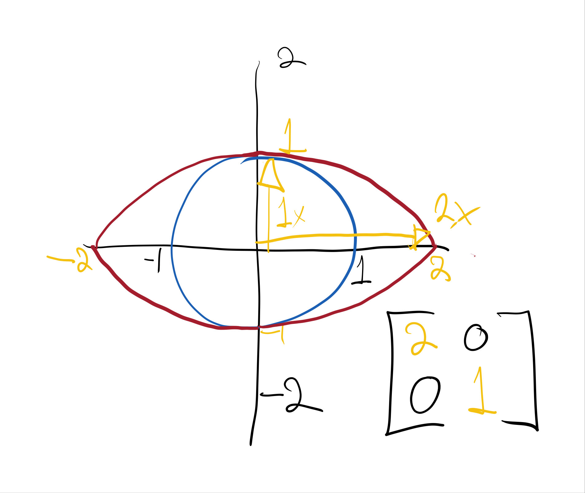
If our matrix wasn’t diagonal we’d stretch the unit circle along different axes that aren’t aligned with the standard x and y axes. This transforms the circle by first scaling across the x and y axes then rotating the circle. This geometric intuition becomes useful when proving results about Singular Value Decomposition.

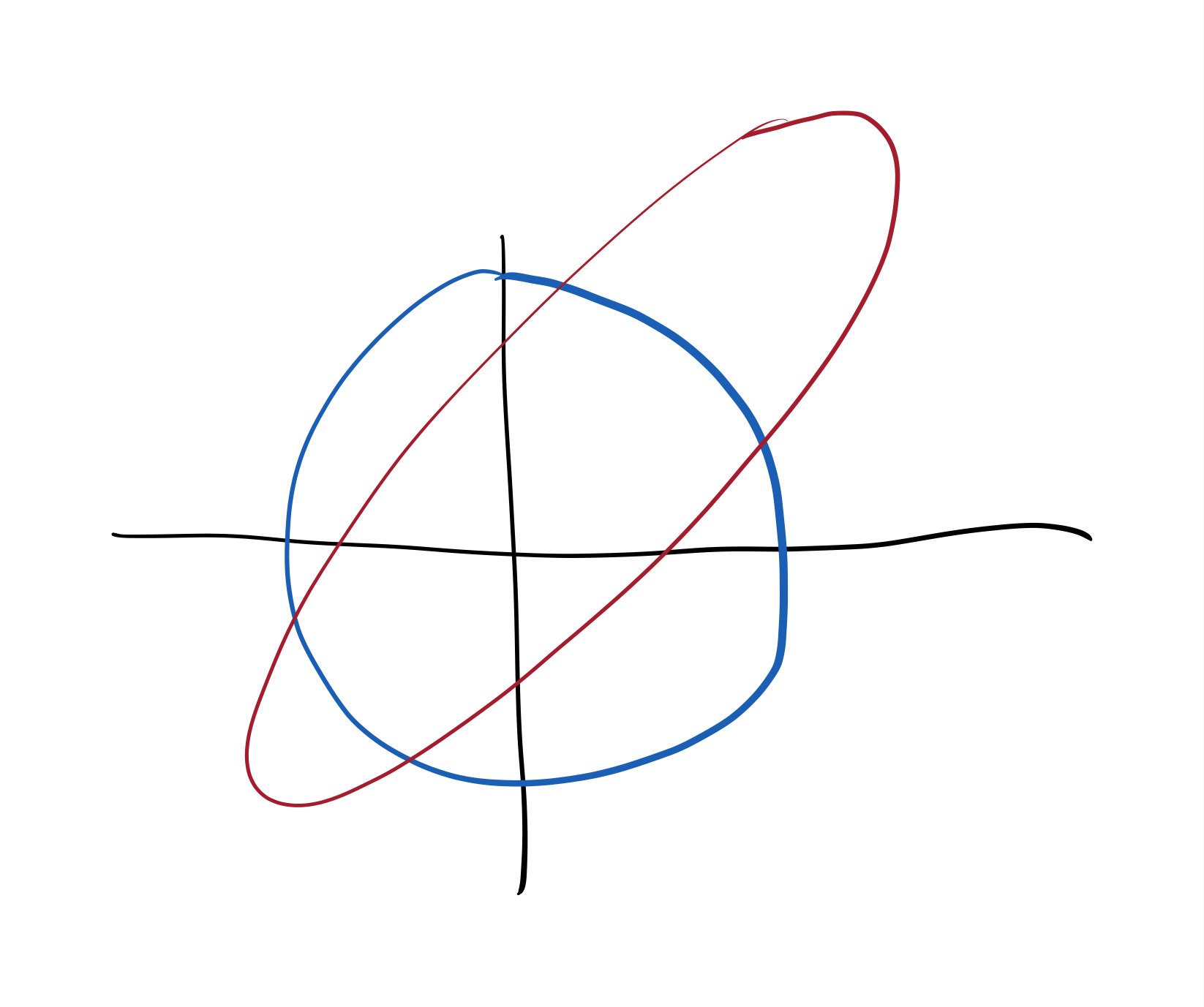
It’s not hard to show that, for diagonal 2x2 matrices, the 2d vector that’s scaled the most is one of the unit vectors aligned with the x and y coordinates. You get this by writing unit vectors as \((\cos \theta, \sin \theta)\). In this case the resulting vector is \((\lambda_1 \cos \theta, \lambda_2\sin \theta)\) then applying some trigonometric identities and working by cases on whether \(\lambda_1 < \lambda_2\).

In higher dimensions we have a similar result by treating it as a simple optimisation problem where the magnitude of the new vector is \(\sqrt{\lambda_1^2 x_1^2 + \lambda_2^2 x_2^2 + \cdots + \lambda_n^2 x_n^2}\). When we do this, we find that the largest scale factor is the largest diagonal entry in the matrix. Which tells us that the matrix norm is \( |\Lambda | = \max_{i} \lambda_i = \lambda_{\max}\)

So for diagonal matrices, we can find the scale factor by finding the largest number on the diagonal. The simplicity of this process makes this really good for us, but we don’t know what \(\Lambda\) is yet which means we can’t use this just yet. The problem of finding \(\Lambda\) and the \( \lambda_i \) is called diagonalisation but unfortunately for us this is generally hard to do.

But we have methods to analytically bound the value of \(\lambda_{\max}\) that are similarly easy to use. One of these methods uses the Gershgorin circle theorem which I’ll walk through next.

Planned: Explicit euler region of stability, gershgorin circle theorem, implicit schemes, Gauss-Seidel

References

[1]: LeVeque, Randall J. Finite difference methods for ordinary and partial differential equations

[2]: Trefethen, Lloyd N., and David Bau. Numerical linear algebra.