Numerically solving recurrence relations in parallel

Learning Julia because it’s trendy

13 Janurary 2025

Given an array of data \(d_i\), its prefix sum is a new array of data where every element of the array is transformed by adding it to the sum of all elements that preceed it. This is basically a cumulative sum where

\[ \operatorname{prefix} (d)_i = \sum_{j=1}^i d_j \]

We can use the prefix sum to estimate CDFs when given relative likelihoods or count data. This is the discrete parallel for integrating over continuous functions.

We can rewrite the definition of the prefix sum slightly and put it in a different form

\[ \begin{align*} \operatorname{prefix}(d)_i &= d_i + \sum_{j = 1}^{i - 1} d_j \\ \operatorname{prefix}(d)_i &= d_ i + \operatorname{prefix}(d)_{i - 1} \\ \end{align*} \]

This form defines the prefix sum in terms of previous values of itself and we can calculate the prefix sum in a simple fashion by sequentially applying its definition

prefix xs = go 0 xs
    where
    go _ [] = []
    go acc (x : xs) = (acc + x) : go (acc + x) xs

This is an instance of what’s called a “scan” or reduction operation. In Julia I could write this iteratively like this

function prefix(X :: AbstractArray{Int64, N}) :: AbstractArray{Int64, N} where N
    result = similar(X, Int64)
    result[1] = X[1]
    for index in 2:length(X)
        result[index] = X[index] + result[index - 1]
    end
    return result
end

But Julia also has a scan function called accumulate so I can also write it like this

array = Vector{Int64}[1, 2, 3, 4, 5]
println(accumulate(+, array))

At a first glance this looks difficult to parallelise since the definition of \(x_i\) depends on the value of \(x_{i-1}\) however we can split our computation of the prefix sum into several steps where each step can be decomposed into tasks that run in parallel to eachother.

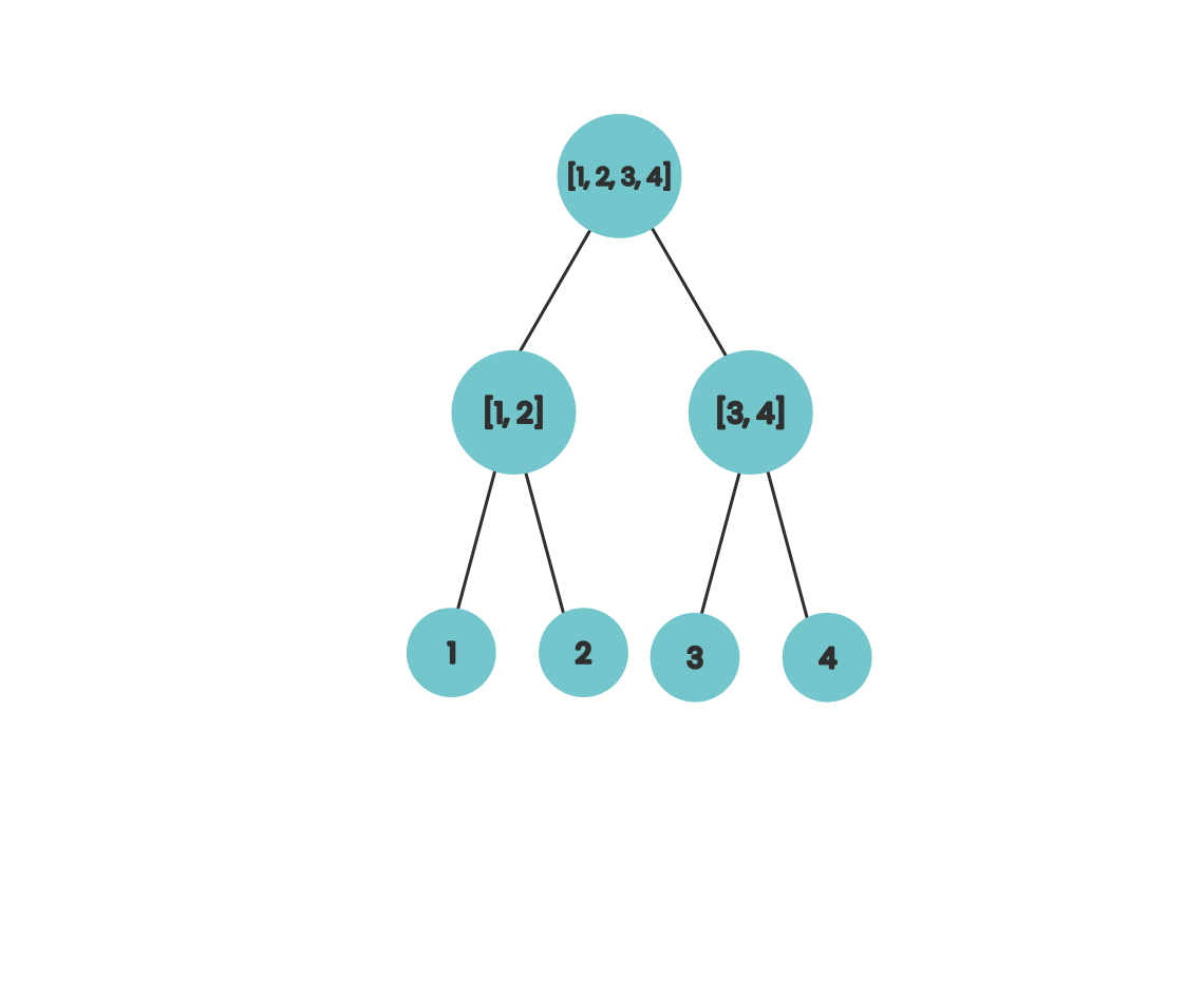
If we wanted to compute the sum of our array in parallel we might use a divide-and-conquer approach where we repeatedly split our array in half and assign the task of calculating the partial sums of our partitions to each of our compute units. As a diagram it looks like this

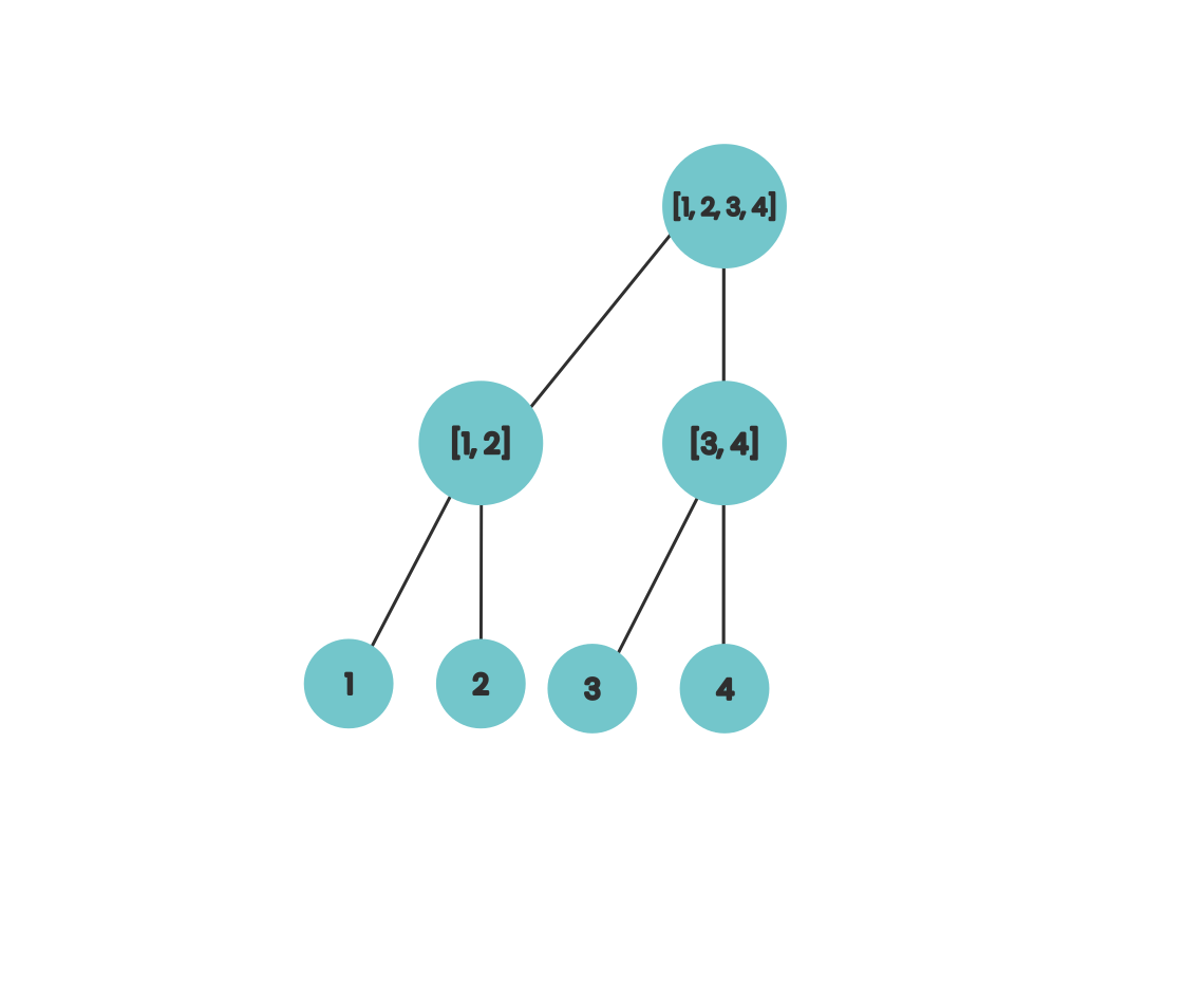
This works because at each step the work a compute unit is doing is independent of the work that other compute units are doing at the same time. If we move our nodes in our diagram a bit to the right we can get a bit of visual intuition for the algorithm that calculates the prefix sums in parallel.

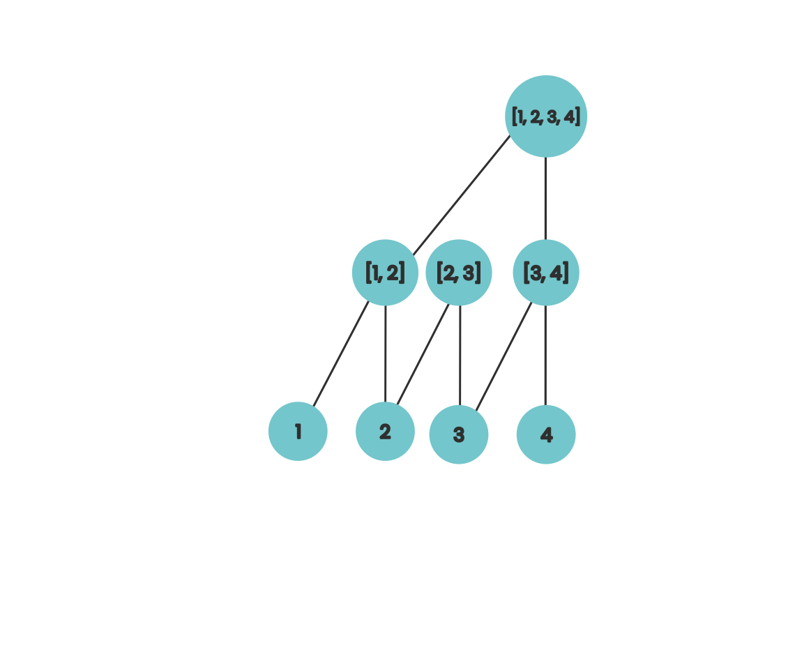
If we associate each of the internal nodes from this tree with the array index it sits on top of then we can interpret each level as computing a portion of the value of the prefix sum for that index. So after the first step, locations 2 and 4 contain the the sum of the final two elements in their prefix. If we do this for numbers that aren’t powers of two then our diagram looks like this

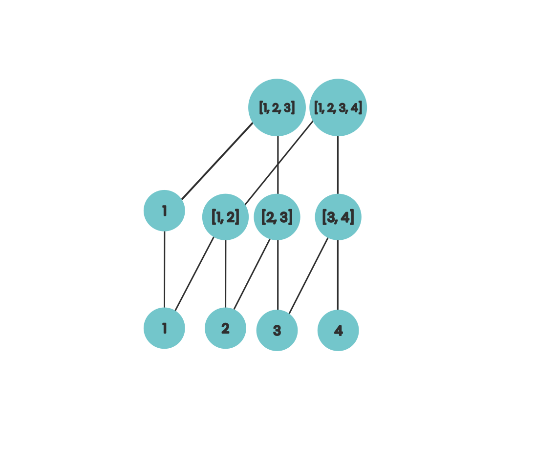
Here we can visually see that after our first step, our array locations have the sum of up to the final 2 elements of its prefix. If we extend this slightly then our diagram looks like this

Here we’re now incremently calculating the prefix sum for each of our array locations using work from the previous step and this is fairly similar to the idea that’s behind how Fenwick trees work.

We can turn this idea into a parallel algorithm. I’m writing this using MPI in Julia since Julia is a language that I’ve been wanting to learn and do a bit more work with for a while

using MPI
MPI.Init()

comm = MPI.COMM_WORLD
rank = MPI.Comm_rank(comm)
size = MPI.Comm_size(comm)

function prefix(X :: AbstractArray{Int64, N}) :: AbstractArray{Int64, N} where N
    result = copy(X)
    broadcast_view = similar(X)

    n = Int64(length(result))
    total_substeps = n
    max_subarray_size = 1

    lookbehind = 1
    for step in 1:Int64(ceil(log2(n)))
        MPI.Bcast!(result, 0, comm)
        workspace = copy(result)

        smallest_valid_index = lookbehind + 1
        total_subtasks = n - smallest_valid_index + 1
        active_cores = min(size, total_subtasks)
        core_is_active = rank < active_cores
        subtasks_per_rank = total_subtasks ÷ active_cores
        if core_is_active
            if rank == active_cores - 1 
                my_subtasks = subtasks_per_rank + (total_subtasks % active_cores)
            else
                my_subtasks = subtasks_per_rank
            end
            start_location = smallest_valid_index + subtasks_per_rank * rank
            end_location = start_location + my_subtasks - 1

            for subtask_delta in 0 : my_subtasks - 1
                location = start_location + subtask_delta
                workspace[location] += result[location - lookbehind]
            end
        end

        for unit in 0 : active_cores - 1
            if unit == active_cores - 1 
                unit_subtasks = subtasks_per_rank + (total_subtasks % active_cores)
            else
                unit_subtasks = subtasks_per_rank
            end

            start_location = smallest_valid_index + subtasks_per_rank * unit
            end_location = start_location + unit_subtasks - 1
            broadcast_view[start_location : end_location] = workspace[start_location : end_location]
            MPI.Bcast!(broadcast_view, unit, comm)
            result[start_location : end_location] = broadcast_view[start_location : end_location]
        end
        MPI.Barrier(comm)
        lookbehind *= 2
    end
    return result
end

array = Int64[1, 2, 3, 4, 5]
result = prefix(array)
if rank == 0
    println(result)
end

Prefix sums are also just a special type of recurrence relation. Recurrence relations come up loads in applied maths: for example, AR models from econometrics.

In general terms, a linear first order recurrence relations \(x_t\) takes the following form

\[ x_t = a_tx_{t - 1} + d_t \]

for coefficients \(a_t\) and data \(d_t\).

So really our prefix sum is just a first-order linear recurrence relation where all \(a_t\) are set to one.

Similar to prefix sums, it’s not immediately obvious how we can parallelise calculating the terms of our recurrence relation. However, we can rewrite our equation like this

\[ \begin{align*} x_t &= a_tx_{t - 1} + d_t \\ &= a_t(a_{t-1} x_{t - 2} + d_{t - 1}) + d_t \\ &= a_ta_{t - 1}x_{t - 2} + a_{t - 1}d_{t - 1} + d_t \\ \end{align*} \]

At a first glance this does’t seem to help us since in this form \(x_t\) still depends on \(x_{t - 2}\), a previous value from the sequence. However we can notice that \(t - 2\) has the same parity as \(t\) so we can have two compute units computing different partitions of our result: one will operate on data with odd indices and one will operate on data with even indices and this generalises for the case where we have more than 2 processors.

Julia was pretty fun to use, the setup and installation was simple and it was very easy to install the MPI bindings. I definitely want to try and use it a bit more in the future.

References

[1]: Hockney, Roger W., and Chris R. Jesshope. Parallel Computers 2: architecture, programming and algorithms. CRC Press, 2019.